Time-varying depths

Some hydrodynamic models (such as SWASH) have time-evolving depth dimensions, for example because they follow the waves on the free surface. Parcels can work with these types of models, but it is a bit involved to set up. That is why we explain here how to run Parcels on FieldSets with time-evolving depth dimensions

from datetime import timedelta as delta
from os import path

import matplotlib.pyplot as plt
import numpy as np
import xarray as xr

from parcels import (
    AdvectionRK4,
    FieldSet,
    JITParticle,
    ParticleFile,
    ParticleSet,
    download_example_dataset,
)

Here, we use sample data from the SWASH model. We first set the filenames and variables

example_dataset_folder = download_example_dataset("SWASH_data")
filenames = f"{example_dataset_folder}/field_*.nc"
variables = {
    "U": "cross-shore velocity",
    "V": "along-shore velocity",
    "depth_u": "time varying depth_u",
}

Now, the first key step when reading time-evolving depth dimensions is that we specify depth as 'not_yet_set' in the dimensions dictionary

dimensions = {
    "U": {"lon": "x", "lat": "y", "depth": "not_yet_set", "time": "t"},
    "V": {"lon": "x", "lat": "y", "depth": "not_yet_set", "time": "t"},
    "depth_u": {"lon": "x", "lat": "y", "depth": "not_yet_set", "time": "t"},
}

Then, after we create the FieldSet object, we set the depth dimension of the relevant Fields to fieldset.depth_u and fieldset.depth_w, using the Field.set_depth_from_field() method

fieldset = FieldSet.from_netcdf(
    filenames, variables, dimensions, mesh="flat", allow_time_extrapolation=True
)
fieldset.U.set_depth_from_field(fieldset.depth_u)
fieldset.V.set_depth_from_field(fieldset.depth_u)

WARNING: Flipping lat data from North-South to South-North. Note that this may lead to wrong sign for meridional velocity, so tread very carefully

Now, we can create a ParticleSet, run those and plot them

pset = ParticleSet(fieldset, JITParticle, lon=9.5, lat=12.5, depth=-0.1)

pfile = pset.ParticleFile("SwashParticles", outputdt=delta(seconds=0.05))

pset.execute(AdvectionRK4, dt=delta(seconds=0.005), output_file=pfile)

INFO: Output files are stored in SwashParticles.zarr.
100%|██████████| 0.25/0.25 [00:00<00:00,  1.61it/s]

ds = xr.open_zarr("SwashParticles.zarr")

plt.plot(ds.lon.T, ds.lat.T, ".-")
plt.show()

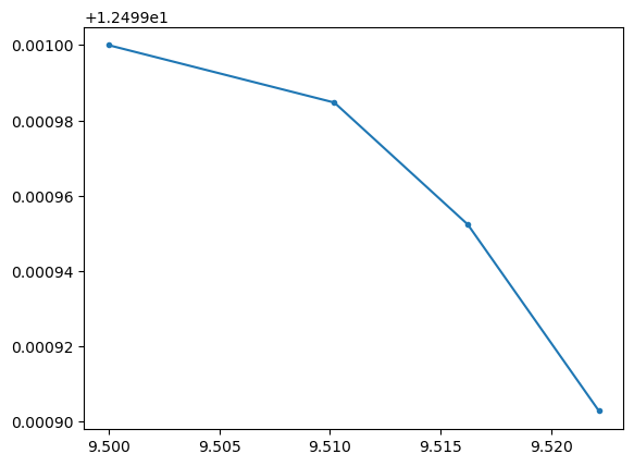
Note that, even though we use 2-dimensional AdvectionRK4, the particle still moves down, because the grid itself moves down