NestedFields

In some applications, you may have access to different fields that each cover only part of the region of interest. Then, you would like to combine them all together. You may also have a field covering the entire region and another one only covering part of it, but with a higher resolution. The set of those fields form what we call nested fields.

It is possible to combine all those fields with kernels, either with different if/else statements depending on particle position.

However, an easier way to work with nested fields in Parcels is to combine all those fields into one NestedField object. The Parcels code will then try to successively interpolate the different fields.

For each Particle, the algorithm is the following:

1. Interpolate the particle onto the first Field in the NestedFields list.

2. If the interpolation succeeds or if an error other than ErrorOutOfBounds is thrown, the function is stopped.

3. If an ErrorOutOfBounds is thrown, try step 1) again with the next Field in the NestedFields list

4. If interpolation on the last Field in the NestedFields list also returns an ErrorOutOfBounds, then the Particle is flagged as OutOfBounds.

This algorithm means that the order of the fields in the ‘NestedField’ matters. In particular, the smallest/finest resolution fields have to be listed before the larger/coarser resolution fields.

Note also that pset.execute() can be much slower on NestedField objects than on normal Fields. This is because the handling of the ErrorOutOfBounds (step 3) happens outside the fast inner-JIT-loop in C; but instead is delt with in the slower python loop around it. This means that especially in cases where particles often move from one nest to another, simulations can become very slow.

This tutorial shows how to use these NestedField with a very idealised example.

import matplotlib.pyplot as plt
import numpy as np
import xarray as xr

import parcels

First define a zonal and meridional velocity field defined on a high resolution (dx = 100m) 2kmx2km grid with a flat mesh. The zonal velocity is uniform and 1 m/s, and the meridional velocity is equal to 0.5 _ cos(lon / 200 _ pi / 2) m/s.

dim = 21
lon = np.linspace(0.0, 2e3, dim, dtype=np.float32)
lat = np.linspace(0.0, 2e3, dim, dtype=np.float32)
lon_g, lat_g = np.meshgrid(lon, lat)
V1_data = np.cos(lon_g / 200 * np.pi / 2)
U1 = parcels.Field("U1", np.ones((dim, dim), dtype=np.float32), lon=lon, lat=lat)
V1 = parcels.Field("V1", V1_data, grid=U1.grid)

Now define the same velocity field on a low resolution (dx = 2km) 20kmx4km grid.

xdim = 11
ydim = 3
lon = np.linspace(-2e3, 18e3, xdim, dtype=np.float32)
lat = np.linspace(-1e3, 3e3, ydim, dtype=np.float32)
lon_g, lat_g = np.meshgrid(lon, lat)
V2_data = np.cos(lon_g / 200 * np.pi / 2)
U2 = parcels.Field("U2", np.ones((ydim, xdim), dtype=np.float32), lon=lon, lat=lat)
V2 = parcels.Field("V2", V2_data, grid=U2.grid)

We now combine those fields into a NestedField and create the fieldset

U = parcels.NestedField("U", [U1, U2])
V = parcels.NestedField("V", [V1, V2])
fieldset = parcels.FieldSet(U, V)

pset = parcels.ParticleSet(fieldset, pclass=parcels.JITParticle, lon=[0], lat=[1000])

output_file = pset.ParticleFile(
    name="NestedFieldParticle.zarr", outputdt=50, chunks=(1, 100)
)

pset.execute(parcels.AdvectionRK4, runtime=14000, dt=10, output_file=output_file)

ds = xr.open_zarr("NestedFieldParticle.zarr")
plt.plot(ds.lon.T, ds.lat.T, ".-")
plt.plot([0, 2e3, 2e3, 0, 0], [0, 0, 2e3, 2e3, 0], c="orange")
plt.plot([-2e3, 18e3, 18e3, -2e3, -2e3], [-1e3, -1e3, 3e3, 3e3, -1e3], c="green");

INFO: Output files are stored in NestedFieldParticle.zarr.
100%|██████████| 14000.0/14000.0 [00:01<00:00, 9625.92it/s]

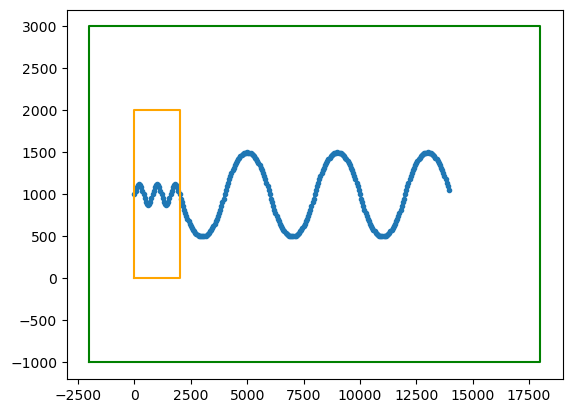
As we observe, there is a change of dynamic at lon=2000, which corresponds to the change of grid.

The analytical solution to the problem:

\begin{align} dx/dt &= 1;\\ dy/dt &= \cos(x \pi/400);\\ \text{with } x(0) &= 0, y(0) = 1000 \end{align}

is

\begin{align} x(t) &= t;\\ y(t) &= 1000 + 400/\pi \sin(t \pi / 400) \end{align}

which is captured by the High Resolution field (orange area) but not the Low Resolution one (green area).

Keep track of the field interpolated

For different reasons, you may want to keep track of the field you have interpolated. You can do that easily by creating another field that share the grid with original fields. Watch out that this operation has a cost of a full interpolation operation.

# Need to redefine fieldset
fieldset = parcels.FieldSet(U, V)

ones_array1 = np.ones((U1.grid.ydim, U1.grid.xdim), dtype=np.float32)
F1 = parcels.Field("F1", ones_array1, grid=U1.grid)

ones_array2 = np.ones((U2.grid.ydim, U2.grid.xdim), dtype=np.float32)
F2 = parcels.Field("F2", 2 * ones_array2, grid=U2.grid)

F = parcels.NestedField("F", [F1, F2])
fieldset.add_field(F)

def SampleNestedFieldIndex(particle, fieldset, time):
    particle.f = fieldset.F[time, particle.depth, particle.lat, particle.lon]


SampleParticle = parcels.JITParticle.add_variable("f", dtype=np.int32)

pset = parcels.ParticleSet(fieldset, pclass=SampleParticle, lon=[1000], lat=[500])
pset.execute(SampleNestedFieldIndex, runtime=1)
print(
    f"Particle ({pset[0].lon:g}, {pset[0].lat:g}) "
    f"interpolates Field #{int(pset[0].f)}"
)

pset[0].lon = 10000
pset.execute(SampleNestedFieldIndex, runtime=1)
print(
    f"Particle ({pset[0].lon:g}, {pset[0].lat:g}) "
    f"interpolates Field #{int(pset[0].f)}"
)

100%|██████████| 1.0/1.0 [00:00<00:00, 528.52it/s]
Particle (1000, 500) interpolates Field #1
100%|██████████| 1.0/1.0 [00:00<00:00, 1368.01it/s]
Particle (1000, 500) interpolates Field #1