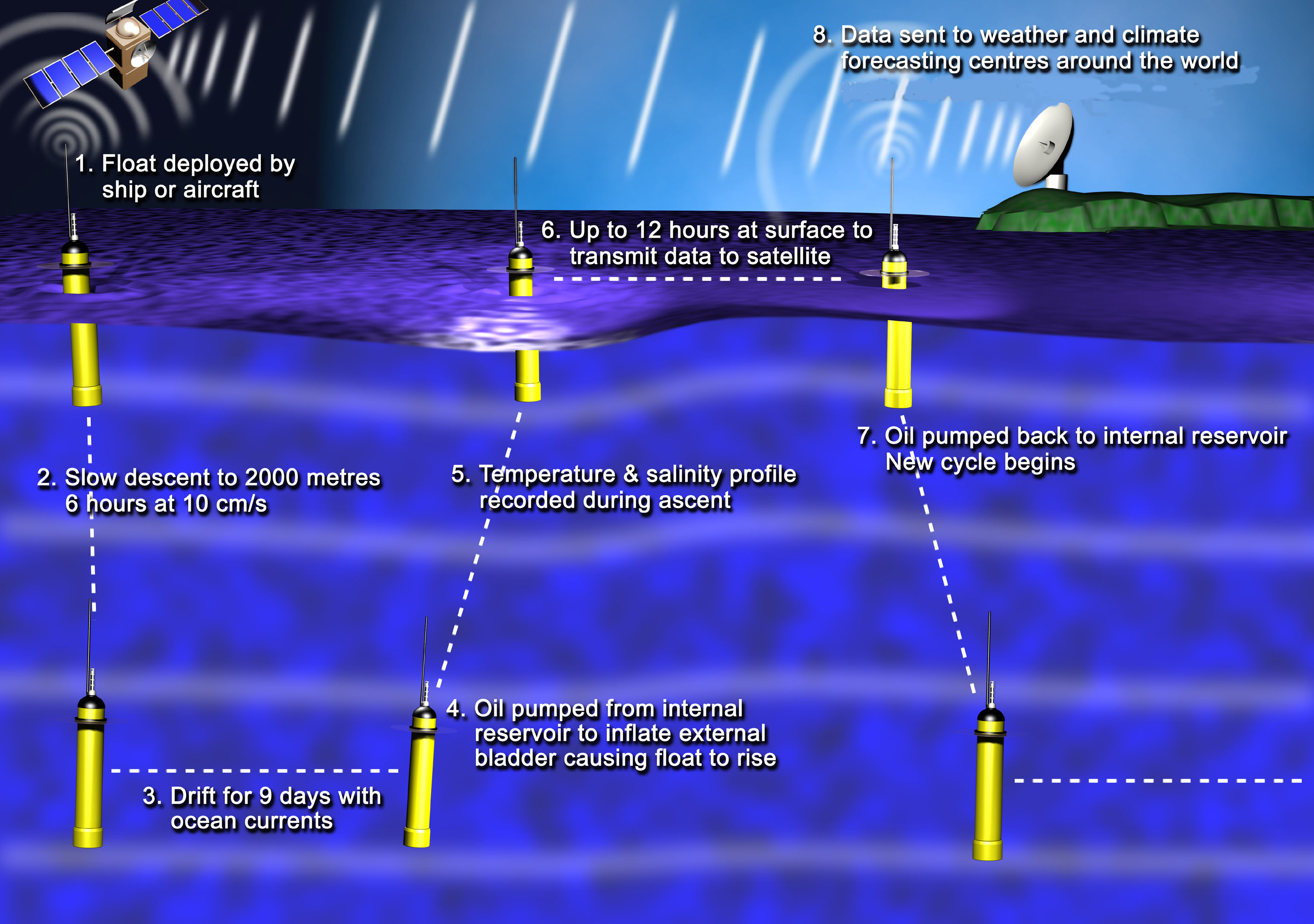
An Argo float

This tutorial shows how simple it is to construct a Kernel in Parcels that mimics the vertical movement of Argo floats.

# Define the new Kernel that mimics Argo vertical movement
def ArgoVerticalMovement(particle, fieldset, time):
    driftdepth = 1000  # maximum depth in m
    maxdepth = 2000  # maximum depth in m
    vertical_speed = 0.10  # sink and rise speed in m/s
    cycletime = 10 * 86400  # total time of cycle in seconds
    drifttime = 9 * 86400  # time of deep drift in seconds

    if particle.cycle_phase == 0:
        # Phase 0: Sinking with vertical_speed until depth is driftdepth
        particle_ddepth += vertical_speed * particle.dt
        if particle.depth + particle_ddepth >= driftdepth:
            particle_ddepth = driftdepth - particle.depth
            particle.cycle_phase = 1

    elif particle.cycle_phase == 1:
        # Phase 1: Drifting at depth for drifttime seconds
        particle.drift_age += particle.dt
        if particle.drift_age >= drifttime:
            particle.drift_age = 0  # reset drift_age for next cycle
            particle.cycle_phase = 2

    elif particle.cycle_phase == 2:
        # Phase 2: Sinking further to maxdepth
        particle_ddepth += vertical_speed * particle.dt
        if particle.depth + particle_ddepth >= maxdepth:
            particle_ddepth = maxdepth - particle.depth
            particle.cycle_phase = 3

    elif particle.cycle_phase == 3:
        # Phase 3: Rising with vertical_speed until at surface
        particle_ddepth -= vertical_speed * particle.dt
        # particle.temp = fieldset.temp[time, particle.depth, particle.lat, particle.lon]  # if fieldset has temperature
        if particle.depth + particle_ddepth <= fieldset.mindepth:
            particle_ddepth = fieldset.mindepth - particle.depth
            # particle.temp = 0./0.  # reset temperature to NaN at end of sampling cycle
            particle.cycle_phase = 4

    elif particle.cycle_phase == 4:
        # Phase 4: Transmitting at surface until cycletime is reached
        if particle.cycle_age > cycletime:
            particle.cycle_phase = 0
            particle.cycle_age = 0

    if particle.state == StatusCode.Evaluate:
        particle.cycle_age += particle.dt  # update cycle_age

And then we can run Parcels with this ‘custom kernel’.

Note that below we use the two-dimensional velocity fields of GlobCurrent, as these are provided as example_data with Parcels.

We therefore assume that the horizontal velocities are the same throughout the entire water column. However, the ArgoVerticalMovement kernel will work on any FieldSet, including from full three-dimensional hydrodynamic data.

If the hydrodynamic data also has a Temperature Field, then uncommenting the lines about temperature will also simulate the sampling of temperature.

from datetime import timedelta

import numpy as np

from parcels import (
    AdvectionRK4,
    FieldSet,
    JITParticle,
    ParticleSet,
    StatusCode,
    Variable,
    download_example_dataset,
)

# Load the GlobCurrent data in the Agulhas region from the example_data
example_dataset_folder = download_example_dataset("GlobCurrent_example_data")
filenames = {
    "U": f"{example_dataset_folder}/20*.nc",
    "V": f"{example_dataset_folder}/20*.nc",
}
variables = {
    "U": "eastward_eulerian_current_velocity",
    "V": "northward_eulerian_current_velocity",
}
dimensions = {"lat": "lat", "lon": "lon", "time": "time"}
fieldset = FieldSet.from_netcdf(filenames, variables, dimensions)
# uppermost layer in the hydrodynamic data
fieldset.mindepth = fieldset.U.depth[0]


# Define a new Particle type including extra Variables
ArgoParticle = JITParticle.add_variables(
    [
        # Phase of cycle:
        # init_descend=0,
        # drift=1,
        # profile_descend=2,
        # profile_ascend=3,
        # transmit=4
        Variable("cycle_phase", dtype=np.int32, initial=0.0),
        Variable("cycle_age", dtype=np.float32, initial=0.0),
        Variable("drift_age", dtype=np.float32, initial=0.0),
        # if fieldset has temperature
        # Variable('temp', dtype=np.float32, initial=np.nan),
    ]
)

# Initiate one Argo float in the Agulhas Current
pset = ParticleSet(
    fieldset=fieldset, pclass=ArgoParticle, lon=[32], lat=[-31], depth=[0]
)

# combine Argo vertical movement kernel with built-in Advection kernel
kernels = [ArgoVerticalMovement, AdvectionRK4]

# Create a ParticleFile object to store the output
output_file = pset.ParticleFile(
    name="argo_float",
    outputdt=timedelta(minutes=15),
    chunks=(1, 500),  # setting to write in chunks of 500 observations
)

# Now execute the kernels for 30 days, saving data every 30 minutes
pset.execute(
    kernels,
    runtime=timedelta(days=30),
    dt=timedelta(minutes=15),
    output_file=output_file,
)

INFO: Output files are stored in argo_float.zarr.
100%|██████████| 2592000.0/2592000.0 [00:20<00:00, 129080.81it/s]

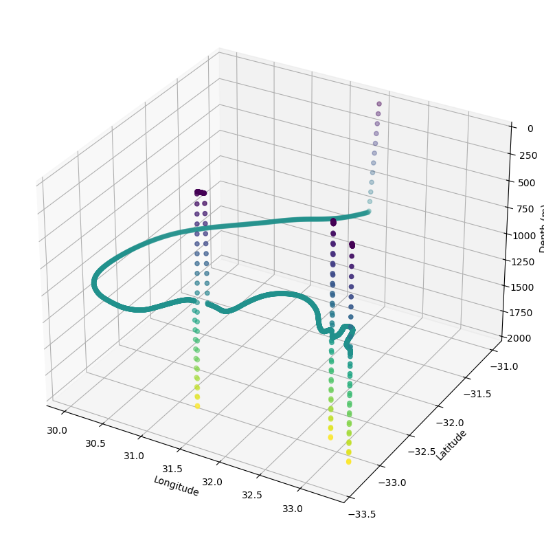
Now we can plot the trajectory of the Argo float with some simple calls to netCDF4 and matplotlib

import matplotlib.pyplot as plt
import xarray as xr
from mpl_toolkits.mplot3d import Axes3D

ds = xr.open_zarr("argo_float.zarr")
x = ds["lon"][:].squeeze()
y = ds["lat"][:].squeeze()
z = ds["z"][:].squeeze()
ds.close()

fig = plt.figure(figsize=(13, 10))
ax = plt.axes(projection="3d")
cb = ax.scatter(x, y, z, c=z, s=20, marker="o")
ax.set_xlabel("Longitude")
ax.set_ylabel("Latitude")
ax.set_zlabel("Depth (m)")
ax.set_zlim(np.max(z), 0)
plt.show()