Interpolation

Parcels support a range of different interpolation methods for tracers, such as temperature. Here, we will show how these work, in an idealised example.

We first import the relevant modules

import matplotlib.pyplot as plt
import numpy as np
from matplotlib import cm

from parcels import FieldSet, JITParticle, ParticleSet

We create a small 2D grid where P is a tracer that we want to interpolate. In each grid cell, P has a random value between 0.1 and 1.1. We then set P[1,1] to 0, which for Parcels specifies that this is a land cell

dims = [5, 4]
dx, dy = 1.0 / dims[0], 1.0 / dims[1]
dimensions = {
    "lat": np.linspace(0.0, 1.0, dims[0], dtype=np.float32),
    "lon": np.linspace(0.0, 1.0, dims[1], dtype=np.float32),
}
data = {
    "U": np.zeros(dims, dtype=np.float32),
    "V": np.zeros(dims, dtype=np.float32),
    "P": np.random.rand(dims[0], dims[1]) + 0.1,
}
data["P"][1, 1] = 0.0
fieldset = FieldSet.from_data(data, dimensions, mesh="flat")

We create a Particle class that can sample this field

SampleParticle = JITParticle.add_variable("p", dtype=np.float32)


def SampleP(particle, fieldset, time):
    particle.p = fieldset.P[time, particle.depth, particle.lat, particle.lon]

Now, we perform four different interpolation on P, which we can control by setting fieldset.P.interp_method. Note that this can always be done after the FieldSet creation. We store the results of each interpolation method in an entry in the dictionary pset.

pset = {}
interp_methods = ["linear", "linear_invdist_land_tracer", "nearest", "cgrid_tracer"]
for p_interp in interp_methods:
    fieldset.P.interp_method = (
        p_interp  # setting the interpolation method for fieldset.P
    )

    xv, yv = np.meshgrid(np.linspace(0, 1, 8), np.linspace(0, 1, 8))
    pset[p_interp] = ParticleSet(
        fieldset, pclass=SampleParticle, lon=xv.flatten(), lat=yv.flatten()
    )
    pset[p_interp].execute(SampleP, endtime=1, dt=1)

100%|██████████| 1.0/1.0 [00:00<00:00, 639.38it/s]
100%|██████████| 1.0/1.0 [00:00<00:00, 663.66it/s]
100%|██████████| 1.0/1.0 [00:00<00:00, 832.70it/s]
100%|██████████| 1.0/1.0 [00:00<00:00, 532.47it/s]

And then we can show each of the four interpolation methods, by plotting the interpolated values on the Particle locations (circles) on top of the Field values (background colors)

fig, ax = plt.subplots(1, 4, figsize=(18, 5))
for i, p in enumerate(pset.keys()):
    data = fieldset.P.data[0, :, :]
    data[1, 1] = np.nan
    x = np.linspace(-dx / 2, 1 + dx / 2, dims[0] + 1)
    y = np.linspace(-dy / 2, 1 + dy / 2, dims[1] + 1)
    if p == "cgrid_tracer":
        for lat in fieldset.P.grid.lat:
            ax[i].axhline(lat, color="k", linestyle="--")
        for lon in fieldset.P.grid.lon:
            ax[i].axvline(lon, color="k", linestyle="--")
    ax[i].pcolormesh(y, x, data, vmin=0.1, vmax=1.1)
    ax[i].scatter(
        pset[p].lon, pset[p].lat, c=pset[p].p, edgecolors="k", s=50, vmin=0.1, vmax=1.1
    )
    xp, yp = np.meshgrid(fieldset.P.lon, fieldset.P.lat)
    ax[i].plot(xp, yp, "kx")
    ax[i].set_title(f"Using interp_method='{p}'")
plt.show()

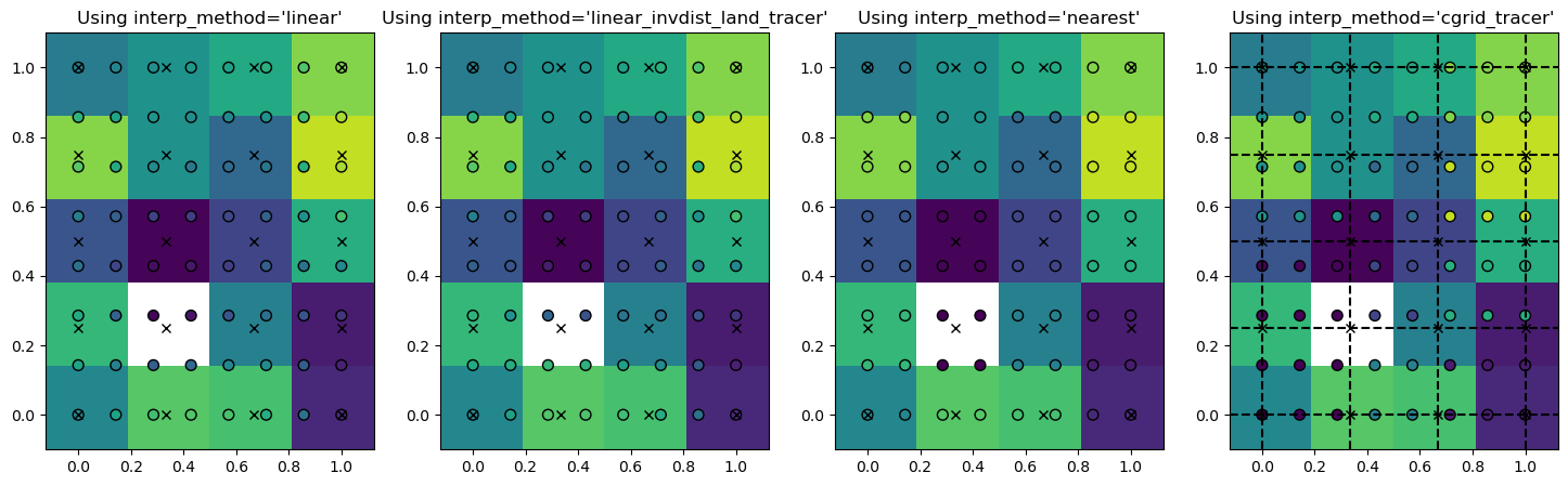
The white box is here the ‘land’ point where the tracer is set to zero and the crosses are the locations of the grid points. As you see, the interpolated value is always equal to the field value if the particle is exactly on the grid point (circles on crosses).

For interp_method='nearest', the particle values are the same for all particles in a grid cell. They are also the same for interp_method='cgrid_tracer', but the grid cells have then shifted. That is because in a C-grid, the tracer grid cell is on the top-right corner (black dashed lines in right-most panel).

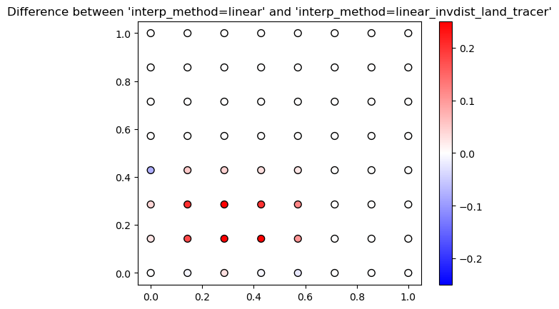
For interp_method='linear_invdist_land_tracer', we see that values are the same as interp_method='linear' for grid cells that don’t border the land point. For grid cells that do border the land cell, the linear_invdist_land_tracer interpolation method gives higher values, as also shown in the difference plot below

plt.scatter(
    pset["linear"].lon,
    pset["linear"].lat,
    c=pset["linear_invdist_land_tracer"].p - pset["linear"].p,
    edgecolors="k",
    s=50,
    cmap=cm.bwr,
    vmin=-0.25,
    vmax=0.25,
)
plt.colorbar()
plt.title(
    "Difference between 'interp_method=linear' "
    "and 'interp_method=linear_invdist_land_tracer'"
)
plt.show()

So in summary, Parcels has four different interpolation schemes for tracers:

1. interp_method=linear: compute linear interpolation

2. interp_method=linear_invdist_land_tracer: compute linear interpolation except near land (where field value is zero). In that case, inverse distance weighting interpolation is computed, weighting by squares of the distance.

3. interp_method=nearest: return nearest field value

4. interp_method=cgrid_tracer: return nearest field value supposing C cells