Quickstart to Parcels

Welcome to a quick tutorial on Parcels. This is meant to get you started with the code, and give you a flavour of some of the key features of Parcels.

In this tutorial, we will first cover how to run a set of particles from a very simple idealised field. We will show how easy it is to run particles in time-backward mode. Then, we will show how to add custom behaviour to the particles. Then we will show how to run particles in a set of NetCDF files from external data. Then we will show how to use particles to sample a field such as temperature or sea surface height. And finally, we will show how to write a kernel that tracks the distance travelled by the particles.

Let’s start with importing the relevant modules. The key ones are all in the parcels package.

import math
from datetime import timedelta
from operator import attrgetter

import matplotlib.pyplot as plt
import numpy as np
import trajan as ta
import xarray as xr
from IPython.display import HTML
from matplotlib.animation import FuncAnimation

from parcels import (
    AdvectionRK4,
    FieldSet,
    JITParticle,
    ParticleSet,
    Variable,
    download_example_dataset,
)

Running particles in an idealised field

The first step to running particles with Parcels is to define a FieldSet object, which is simply a collection of hydrodynamic fields. In this first case, we use a simple flow of two idealised moving eddies. That field can be downloaded using the download_example_dataset() function that comes with Parcels. Since we know that the files are in what’s called Parcels FieldSet format, we can call these files using the function FieldSet.from_parcels().

example_dataset_folder = download_example_dataset("MovingEddies_data")

fieldset = FieldSet.from_parcels(f"{example_dataset_folder}/moving_eddies")

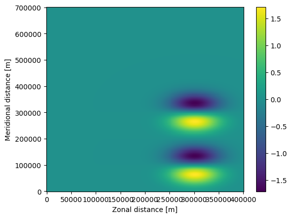
The fieldset can then be visualized with e.g. matplotlib.pyplot.pcolormesh(). To show the zonal velocity (U), give the commands below. Note that we first have to load the fieldset with fieldset.computeTimeChunk() to load the first time frame of the fieldset.

fieldset.computeTimeChunk()

plt.pcolormesh(fieldset.U.grid.lon, fieldset.U.grid.lat, fieldset.U.data[0, :, :])
plt.xlabel("Zonal distance [m]")
plt.ylabel("Meridional distance [m]")
plt.colorbar()
plt.show()

The next step is to define a ParticleSet. In this case, we start 2 particles at locations (330km, 100km) and (330km, 280km) using the from_list constructor method, that are advected on the fieldset we defined above. Note that we use JITParticle as pclass, because we will be executing the advection in JIT (Just-In-Time) mode. The alternative is to run in scipy mode, in which case pclass is ScipyParticle

pset = ParticleSet.from_list(
    fieldset=fieldset,  # the fields on which the particles are advected
    pclass=JITParticle,  # the type of particles (JITParticle or ScipyParticle)
    lon=[3.3e5, 3.3e5],  # a vector of release longitudes
    lat=[1e5, 2.8e5],  # a vector of release latitudes
)

Print the ParticleSet to see where they start

print(pset)

P[0](lon=330000.000000, lat=100000.000000, depth=0.000000, time=not_yet_set)
P[1](lon=330000.000000, lat=280000.000000, depth=0.000000, time=not_yet_set)

This output shows for each particle the (longitude, latitude, depth, time). Note that in this case the time is not_yet_set, that is because we didn’t specify a time when we defined the pset.

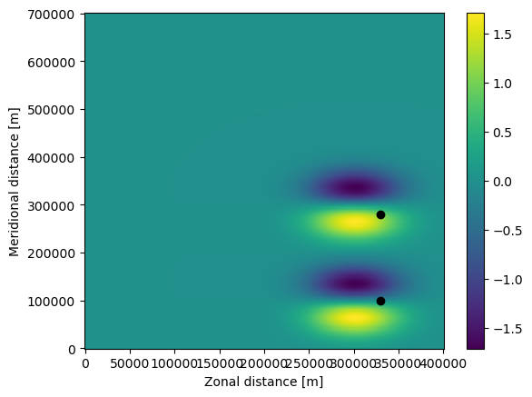
To plot the positions of these particles on the zonal velocity, use the following command

plt.pcolormesh(fieldset.U.grid.lon, fieldset.U.grid.lat, fieldset.U.data[0, :, :])
plt.xlabel("Zonal distance [m]")
plt.ylabel("Meridional distance [m]")
plt.colorbar()

plt.plot(pset.lon, pset.lat, "ko")
plt.show()

The final step is to run (or ‘execute’) the ParticelSet. We run the particles using the AdvectionRK4 kernel, which is a 4th order Runge-Kutte implementation that comes with Parcels. We run the particles for 6 days (using the timedelta function from datetime), at an RK4 timestep of 5 minutes. We store the trajectory information at an interval of 1 hour in a file called EddyParticles.zarr. Because time was not_yet_set, the particles will be advected from the first date available in the fieldset, which is the default behaviour.

output_file = pset.ParticleFile(
    name="EddyParticles.zarr",  # the file name
    outputdt=timedelta(hours=1),  # the time step of the outputs
)
pset.execute(
    AdvectionRK4,  # the kernel (which defines how particles move)
    runtime=timedelta(days=6),  # the total length of the run
    dt=timedelta(minutes=5),  # the timestep of the kernel
    output_file=output_file,
)

INFO: Output files are stored in EddyParticles.zarr.
100%|██████████| 518400.0/518400.0 [00:03<00:00, 172443.78it/s]

The code should have run, which can be confirmed by printing and plotting the ParticleSet again

print(pset)

plt.pcolormesh(fieldset.U.grid.lon, fieldset.U.grid.lat, fieldset.U.data[0, :, :])
plt.xlabel("Zonal distance [m]")
plt.ylabel("Meridional distance [m]")
plt.colorbar()

plt.plot(pset.lon, pset.lat, "ko")
plt.show()

P[0](lon=226905.562500, lat=82515.218750, depth=0.000000, time=518100.000000)
P[1](lon=260835.125000, lat=320403.343750, depth=0.000000, time=518100.000000)

Note that both the particles (the black dots) and the U field have moved in the plot above. Also, the time of the particles is now 518400 seconds, which is 6 days.

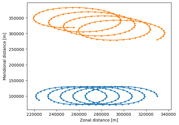
The trajectories in the EddyParticles.zarr file can be quickly plotted using xr.open_zarr() (note that the lon and lat arrays need to be transposed with .T).

ds = xr.open_zarr("EddyParticles.zarr")

plt.plot(ds.lon.T, ds.lat.T, ".-")
plt.xlabel("Zonal distance [m]")
plt.ylabel("Meridional distance [m]")
plt.show()

Using the FuncAnimation() method, we can show the trajectories as an animation and watch the particles go!

%%capture
fig = plt.figure(figsize=(7, 5), constrained_layout=True)
ax = fig.add_subplot()

ax.set_ylabel("Meridional distance [m]")
ax.set_xlabel("Zonal distance [m]")
ax.set_xlim(0, 4e5)
ax.set_ylim(0, 7e5)

# show only every fifth output (for speed in creating the animation)
timerange = np.unique(ds["time"].values)[::5]

# Indices of the data where time = 0
time_id = np.where(ds["time"] == timerange[0])

sc = ax.scatter(ds["lon"].values[time_id], ds["lat"].values[time_id])

t = str(timerange[0].astype("timedelta64[h]"))
title = ax.set_title(f"Particles at t = {t}")


def animate(i):
    t = str(timerange[i].astype("timedelta64[h]"))
    title.set_text(f"Particles at t = {t}")

    time_id = np.where(ds["time"] == timerange[i])
    sc.set_offsets(np.c_[ds["lon"].values[time_id], ds["lat"].values[time_id]])


anim = FuncAnimation(fig, animate, frames=len(timerange), interval=100)

HTML(anim.to_jshtml())

Once Loop Reflect

Running particles in backward time

Running particles in backward time is extremely simple: just provide a dt < 0.

output_file = pset.ParticleFile(
    name="EddyParticles_Bwd.zarr",  # the file name
    outputdt=timedelta(hours=1),  # the time step of the outputs
)
pset.execute(
    AdvectionRK4,
    dt=-timedelta(minutes=5),  # negative timestep for backward run
    runtime=timedelta(days=6),  # the run time
    output_file=output_file,
)

INFO: Output files are stored in EddyParticles_Bwd.zarr.
100%|██████████| 518400.0/518400.0 [00:02<00:00, 176426.86it/s]

Now print the particles again, and see that they (except for some round-off errors) returned to their original position

print(pset)

plt.pcolormesh(fieldset.U.grid.lon, fieldset.U.grid.lat, fieldset.U.data[0, :, :])
plt.xlabel("Zonal distance [m]")
plt.ylabel("Meridional distance [m]")
plt.colorbar()

plt.plot(pset.lon, pset.lat, "ko")
plt.show()

P[0](lon=329983.281250, lat=100495.609375, depth=0.000000, time=300.000000)
P[1](lon=330289.968750, lat=280418.906250, depth=0.000000, time=300.000000)

Adding a custom behaviour kernel

A key feature of Parcels is the ability to quickly create very simple kernels, and add them to the execution. Kernels are little snippets of code that are run during exection of the particles.

In this example, we’ll create a simple kernel where particles obtain an extra 2 m/s westward velocity after 1 day. Of course, this is not very realistic scenario, but it nicely illustrates the power of custom kernels.

def WestVel(particle, fieldset, time):
    if time > 86400:
        uvel = -2.0
        particle_dlon += uvel * particle.dt

Note that in the Kernel above, we update particle_dlon, and not particle.lon directly. This is because of the particular way in which particle locations are updated; see also the tutorial on the particle Kernel loop.

Now reset the ParticleSet again, and re-execute. Note that we have now changed the first argument of pset.execute() to be a list of [AdvectionRK4, WestVel].

pset = ParticleSet.from_list(
    fieldset=fieldset, pclass=JITParticle, lon=[3.3e5, 3.3e5], lat=[1e5, 2.8e5]
)

output_file = pset.ParticleFile(
    name="EddyParticles_WestVel.zarr", outputdt=timedelta(hours=1)
)
pset.execute(
    [AdvectionRK4, WestVel],  # simply combine the Kernels in a list
    runtime=timedelta(days=2),
    dt=timedelta(minutes=5),
    output_file=output_file,
)

INFO: Output files are stored in EddyParticles_WestVel.zarr.
100%|██████████| 172800.0/172800.0 [00:00<00:00, 179532.85it/s]

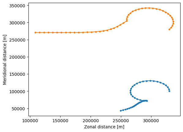
And now plot this new trajectory file

ds = xr.open_zarr("EddyParticles_WestVel.zarr")

plt.plot(ds.lon.T, ds.lat.T, ".-")
plt.xlabel("Zonal distance [m]")
plt.ylabel("Meridional distance [m]")
plt.show()

Reading in data from arbritrary NetCDF files

In most cases, you will want to advect particles within pre-computed velocity fields. If these velocity fields are stored in NetCDF format, it is fairly easy to load them into the FieldSet.from_netcdf() function.

The examples directory contains a set of GlobCurrent files of the region around South Africa.

First, define the names of the files containing the zonal (U) and meridional (V) velocities. You can use wildcards (*) and the filenames for U and V can be the same (as in this case)

example_dataset_folder = download_example_dataset("GlobCurrent_example_data")

filenames = {
    "U": f"{example_dataset_folder}/20*.nc",
    "V": f"{example_dataset_folder}/20*.nc",
}

Then, define a dictionary of the variables (U and V) and dimensions (lon, lat and time; note that in this case there is no depth because the GlobCurrent data is only for the surface of the ocean)

variables = {
    "U": "eastward_eulerian_current_velocity",
    "V": "northward_eulerian_current_velocity",
}
dimensions = {"lat": "lat", "lon": "lon", "time": "time"}

Finally, read in the fieldset using the FieldSet.from_netcdf function with the above-defined filenames, variables and dimensions

fieldset = FieldSet.from_netcdf(filenames, variables, dimensions)

Now define a ParticleSet, in this case with 5 particle starting on a line between (28E, 33S) and (30E, 33S) using the ParticleSet.from_line constructor method

pset = ParticleSet.from_line(
    fieldset=fieldset,
    pclass=JITParticle,
    size=5,  # releasing 5 particles
    start=(28, -33),  # releasing on a line: the start longitude and latitude
    finish=(30, -33),  # releasing on a line: the end longitude and latitude
)

And finally execute the ParticleSet for 10 days using 4th order Runge-Kutta

output_file = pset.ParticleFile(
    name="GlobCurrentParticles.zarr", outputdt=timedelta(hours=6)
)
pset.execute(
    AdvectionRK4,
    runtime=timedelta(days=10),
    dt=timedelta(minutes=5),
    output_file=output_file,
)

INFO: Output files are stored in GlobCurrentParticles.zarr.
100%|██████████| 864000.0/864000.0 [00:00<00:00, 1072517.72it/s]

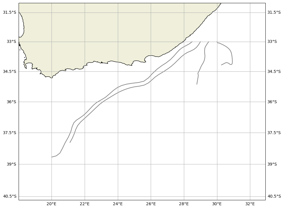
Because the GlobCurrent data represents the ‘real’ ocean, we can use the trajan package to visualize this simulation. Use ds.traj.plot() to plot the trajectories

ds = xr.open_zarr("GlobCurrentParticles.zarr")
ds.traj.plot(margin=2)
plt.show()

Sampling a Field with Particles

One typical use case of particle simulations is to sample a Field (such as temperature, vorticity or sea surface hight) along a particle trajectory. In Parcels, this is very easy to do, with a custom Kernel.

Let’s read in another example, the flow around a Peninsula (see Fig 2.2.3 in this document), and this time also load the Pressure (P) field, using extra_fields={'P': 'P'}. Note that, because this flow does not depend on time, we need to set allow_time_extrapolation=True when reading in the fieldset.

example_dataset_folder = download_example_dataset("Peninsula_data")
fieldset = FieldSet.from_parcels(
    f"{example_dataset_folder}/peninsula",
    extra_fields={"P": "P"},
    allow_time_extrapolation=True,
)

Now define a new Particle class that has an extra Variable: the pressure. This particle.p can be used to store the values of the fieldset.P field at the particle locations.

SampleParticle = JITParticle.add_variable("p")

Note that if you get a AttributeError: type object 'JITParticle' has no attribute 'add_variables' error, you are probably using an old version of Parcels. Please update to the latest version of Parcels using conda update -c conda-forge parcels.

Alternatively, you can refer to the Parcels v3.0.1 documentation, which does not use the new ParticleSet.add_variables() method introduced in Parcels v3.0.2.

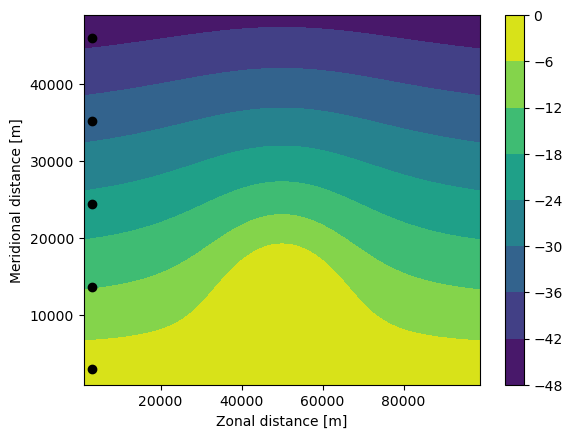
Now define a ParticleSet using the from_line method also used above in the GlobCurrent data. Plot the pset on top of a contour plot of the P field

pset = ParticleSet.from_line(
    fieldset=fieldset,
    pclass=SampleParticle,
    start=(3000, 3000),
    finish=(3000, 46000),
    size=5,
    time=0,
)

plt.contourf(fieldset.P.grid.lon, fieldset.P.grid.lat, fieldset.P.data[0, :, :])
plt.xlabel("Zonal distance [m]")
plt.ylabel("Meridional distance [m]")
plt.colorbar()

plt.plot(pset.lon, pset.lat, "ko")
plt.show()

Now create a custom function that samples the fieldset.P field at the particle location.

def SampleP(particle, fieldset, time):
    """Custom function that samples fieldset.P at particle location"""
    particle.p = fieldset.P[time, particle.depth, particle.lat, particle.lon]

Now, execute the pset with a combination of the AdvectionRK4 and SampleP kernels

output_file = pset.ParticleFile(
    name="PeninsulaPressure.zarr", outputdt=timedelta(hours=1)
)
pset.execute(
    [AdvectionRK4, SampleP],  # list of kernels to be executed
    runtime=timedelta(hours=20),
    dt=timedelta(minutes=5),
    output_file=output_file,
)

INFO: Output files are stored in PeninsulaPressure.zarr.
100%|██████████| 72000.0/72000.0 [00:00<00:00, 143717.52it/s]

Now, plot the particle trajectories on top of the P field, colored by the sampled pressure. As you can see, the dots with black edges are the same color as the background pressure field, which means that the sampling worked!

ds = xr.open_zarr("PeninsulaPressure.zarr")

plt.contourf(fieldset.P.grid.lon, fieldset.P.grid.lat, fieldset.P.data[0, :, :])
plt.xlabel("Zonal distance [m]")
plt.ylabel("Meridional distance [m]")
plt.colorbar()

plt.scatter(ds.lon, ds.lat, c=ds.p, s=30, cmap="viridis", edgecolors="k")
plt.show()

And see that these pressure values p are (within roundoff errors) the same as the pressure values before the execution of the kernels. The particles thus stay on isobars!

Calculating distance travelled

As a second example of what custom kernels can do, we will now show how to create a kernel that logs the total distance that particles have travelled.

First, we need to add three extra variables to the Particle Class. The distance variable will be written to output, but the auxiliary variables prev_lon and prev_lat won’t be written to output (can be controlled using the to_write keyword).

extra_vars = [
    Variable("distance", initial=0.0, dtype=np.float32),
    Variable("prev_lon", dtype=np.float32, to_write=False, initial=attrgetter("lon")),
    Variable("prev_lat", dtype=np.float32, to_write=False, initial=attrgetter("lat")),
]

DistParticle = JITParticle.add_variables(extra_vars)

Now define a new function TotalDistance that calculates the sum of Euclidean distances between the old and new locations in each RK4 step

def TotalDistance(particle, fieldset, time):
    """Calculate the distance in latitudinal direction
    (using 1.11e2 kilometer per degree latitude)"""
    lat_dist = (particle.lat - particle.prev_lat) * 1.11e2
    lon_dist = (
        (particle.lon - particle.prev_lon)
        * 1.11e2
        * math.cos(particle.lat * math.pi / 180)
    )
    # Calculate the total Euclidean distance travelled by the particle
    particle.distance += math.sqrt(math.pow(lon_dist, 2) + math.pow(lat_dist, 2))

    # Set the stored values for next iteration
    particle.prev_lon = particle.lon
    particle.prev_lat = particle.lat

Note: here it is assumed that the latitude and longitude are measured in degrees North and East, respectively. However, some datasets (e.g. the MovingEddies used above) give them measured in (kilo)meters, in which case we must not include the factor 1.11e2.

We will run the TotalDistance function on a ParticleSet containing the five particles within the GlobCurrent fieldset from above. Note that pclass=DistParticle in this case.

example_dataset_folder = download_example_dataset("GlobCurrent_example_data")
filenames = {
    "U": f"{example_dataset_folder}/20*.nc",
    "V": f"{example_dataset_folder}/20*.nc",
}
variables = {
    "U": "eastward_eulerian_current_velocity",
    "V": "northward_eulerian_current_velocity",
}
dimensions = {"lat": "lat", "lon": "lon", "time": "time"}
fieldset = FieldSet.from_netcdf(filenames, variables, dimensions)
pset = ParticleSet.from_line(
    fieldset=fieldset, pclass=DistParticle, size=5, start=(28, -33), finish=(30, -33)
)

Again define a new kernel to include the function written above and execute the ParticleSet.

pset.execute(
    [AdvectionRK4, TotalDistance],  # list of kernels to be executed
    runtime=timedelta(days=6),
    dt=timedelta(minutes=5),
    output_file=pset.ParticleFile(
        name="GlobCurrentParticles_Dist.zarr", outputdt=timedelta(hours=1)
    ),
)

INFO: Output files are stored in GlobCurrentParticles_Dist.zarr.
100%|██████████| 518400.0/518400.0 [00:03<00:00, 136275.28it/s]

And finally print the distance in km that each particle has travelled (note that this is also stored in the EddyParticles_Dist.zarr file)

print([p.distance for p in pset])

[13.197482, 640.92773, 543.45953, 183.60716, 172.74182]