Parcels structure overview

The flexibility of Parcels allows for a wide range of applications and to build complex simulations. In order to help structuring your code, this tutorial describes the structure that a Parcels script uses.

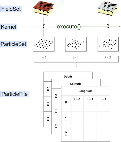
Code that uses Parcels is generally build up from four different components:

1. FieldSet. Load and set up the fields. These can be velocity fields that are used to advect the particles, but it can also be e.g. temperature.

2. ParticleSet. Define the type of particles. Also additional Variables can be added to the particles (e.g. temperature, to keep track of the temperature that particles experience).

3. Kernels. Define and compile kernels. Kernels perform some specific operation on the particles every time step (e.g. interpolate the temperature from the temperature field to the particle location).

4. Execution and output. Execute the simulation and write and store the output in a NetCDF file.

We discuss each component in more detail below.

1. FieldSet

Parcels provides a framework to simulate the movement of particles within an existing flow field environment. To start a parcels simulation we must define this environment with the FieldSet class. The minimal requirements for this Fieldset are that it must contain the 'U' and 'V' fields: the 2D hydrodynamic data that will move the particles in a horizontal direction. Additionally, it can contain e.g. a temperature or vertical flow field.

A fieldset can be loaded with FieldSet.from_netcdf, if the model output with the fields is written in NetCDF files. This function requires filenames, variables and dimensions.

In this example, we only load the 'U' and 'V' fields, which represent the zonal and meridional flow velocity. First, fname points to the location of the model output.

from parcels import download_example_dataset

example_dataset_folder = download_example_dataset("GlobCurrent_example_data")
fname = f"{example_dataset_folder}/*.nc"
filenames = {"U": fname, "V": fname}

Second, we have to specify the 'U' and 'V' variable names, as given by the NetCDF files.

variables = {
    "U": "eastward_eulerian_current_velocity",
    "V": "northward_eulerian_current_velocity",
}

Third, we specify the names of the variable dimensions, as given by the NetCDF files.

# In the GlobCurrent data the dimensions are also called 'lon', 'lat' and 'time
dimensions = {
    "U": {"lat": "lat", "lon": "lon", "time": "time"},
    "V": {"lat": "lat", "lon": "lon", "time": "time"},
}

Finally, we load the fieldset.

from parcels import FieldSet

fieldset = FieldSet.from_netcdf(filenames, variables, dimensions)

For more advanced tutorials on creating FieldSets:

• Implement periodic boundaries

• How to interpolate field data for different fields

• Converting units in the field data

• Working around incompatible time coordinates

If you are working with field data on different grids:

• Grid indexing on different grids

• Load field data from Curvilinear grids

• Load field data from 3D C-grids

If you want to combine different velocity fields:

• Add different velocity fields in a SummedField

• Nest velocity fields of different regions or resolutions in a NestedField

2. ParticleSet

Once the environment has a FieldSet object, you can start defining your particles in a ParticleSet object. This object requires:

1. The FieldSet object in which the particles will be released.

2. The type of Particle: Either a JITParticle or ScipyParticle.

3. Initial conditions for each Variable defined in the Particle, most notably the release locations in lon and lat.

from parcels import JITParticle, ParticleSet, Variable

# Define a new particle class


class AgeParticle(JITParticle):  # It is a JIT particle
    age = Variable("age", initial=0)  # Variable 'age' is added with initial value 0.


pset = ParticleSet(
    fieldset=fieldset,  # the fields that the particleset uses
    pclass=AgeParticle,  # define the type of particle
    lon=29,  # release longitude
    lat=-33,  # release latitude
)

For more advanced tutorials on how to setup your ParticleSet:

• Releasing particles at different times

• The difference between JITParticles and ScipyParticles

For more information on how to implement Particle types with specific behaviour, see the section on writing your own kernels.

3. Kernels

Kernels are little snippets of code, which are applied to every particle in the ParticleSet, for every time step during a simulation. Basic kernels are included in Parcels, among which several types of advection kernels. AdvectionRK4 is the main advection kernel for two-dimensional advection, which is also used in this example.

One can also write custom kernels, to add certain types of ‘behaviour’ to the particles. Kernels can then be combined with the + operator (where at least one of the kernels needs to be cast to a pset.Kernel() object), or by creating a list of the kernels. Note that the kernels are executed in order.

# load basic advection kernels
from parcels import AdvectionRK4

# Create a custom kernel which displaces each particle southward


def NorthVel(particle, fieldset, time):
    if time > 10 * 86400 and time < 10.2 * 86400:
        vvel = -1e-4
        particle.lat += vvel * particle.dt


# Create a custom kernel which keeps track of the particle age (minutes)


def Age(particle, fieldset, time):
    particle.age += particle.dt / 3600


# define all kernels to be executed on particles using an (ordered) list
kernels = [Age, NorthVel, AdvectionRK4]

Some key limitations exist to the Kernels that everyone who wants to write their own should be aware of:

• Every Kernel must be a function with the following (and only those) arguments: (particle, fieldset, time)

• In order to run successfully in JIT mode, Kernel definitions can only contain the following types of commands:

  • Basic arithmetical operators (+, -, *, /, **) and assignments (=).

  • Basic logical operators (<, ==, !=, >, &, |). Note that you can use a statement like particle.lon != particle.lon to check if particle.lon is NaN (since math.nan != math.nan).

  • if and while loops, as well as break statements. Note that for-loops are not supported in JIT mode.

  • Interpolation of a Field from the FieldSet at a [time, depth, lat, lon] point, using square brackets notation. For example, to interpolate the zonal velocity (U) field at the particle location, use the following statement: value = fieldset.U[time, particle.depth, particle.lat, particle.lon]

  • Functions from the math standard library and from the custom ParcelsRandom library.

  • Simple print statements, such as:

    • print("Some print")

    • print(particle.lon)

    • print(f"particle id: {particle.id}")

    • print(f"lon: {particle.lon}, lat: {particle.lat}")

  • Local variables can be used in Kernels, and these variables will be accessible in all concatenated Kernels. Note that these local variables are not shared between particles, and also not between time steps.

  • Note that one has to be careful with writing kernels for vector fields on Curvilinear grids. While Parcels automatically rotates the U and V field when necessary, this is not the case for for example wind data. In that case, a custom rotation function will have to be written.

For more advanced tutorials on writing custom kernels that work on custom particles:

• Sample other fields like temperature.

• Mimic the behaviour of ARGO floats.

• Adding diffusion to approximate subgrid-scale processes and unresolved physics.

• Converting between units in m/s and degree/s.

4. Execution and output

The final part executes the simulation, given the ParticleSet, FieldSet and Kernels, that have been defined in the previous steps. If you like to store the particle data generated in the simulation, you define the ParticleFile to which the output of the kernel execution will be written. Then, on the ParticleSet you have defined, you can use the method ParticleSet.execute() which requires the following arguments:

1. The kernels to be executed.

2. The runtime defining how long the execution loop runs. Alternatively, you may define the endtime at which the execution loop stops.

3. The timestep dt at which to execute the kernels.

4. (Optional) The ParticleFile object to write the output to.

output_file = pset.ParticleFile(
    name="GCParticles.zarr",  # the name of the output file
    outputdt=3600,  # the time period between consecutive out output steps
    chunks=(1, 10),  # the chunking of the output file (number of particles, timesteps)
)

pset.execute(
    kernels,  # the kernel (which defines how particles move)
    runtime=86400 * 24,  # the total length of the run in seconds
    dt=300,  # the timestep of the kernel in seconds
    output_file=output_file,
)

INFO: Compiled ArrayAgeParticleAgeNorthVelAdvectionRK4 ==> /var/folders/1n/500ln6w97859_nqq86vwpl000000gr/T/parcels-504/libaf3202ef8aa79577647d9631e4f42fe7_0.so

Note the use of the chunks argument in the pset.ParticleFile() above. This controls the ‘chunking’ of the output file, which is a way to optimize the writing of the output file. See also the advanced output in zarr format tutorial for more information on this. It is worth to optimise this parameter in your runs, as it can significantly speed up the writing of the output file and thus the runtime of pset.execution().

After running your simulation, you probably want to analyse the output. You can use the `trajan <https://opendrift.github.io/trajan/index.html>`__ package for some simple plotting. However, we recommend you write your own code to analyse your specific output and you can probably separate the analysis from the simulation.

For more tutorials on the parcels output:

• How the output is structured and how to start your own analysis