Grid indexing#
Parcels supports Fields on any curvilinear Grid. For velocity Fields (U, V and W), there are some additional restrictions if the Grid is discretized as an Arakawa B- or Arakawa C-grid. That is because under the hood, Parcels uses a specific interpolation scheme for each of these grid types. This is described in Section 2 of Delandmeter and Van Sebille (2019) and summarized below.
The summary is:
For Arakawa B-and C-grids, Parcels requires the locations of the corner points (f-points) of the grid cells for the
dimensionsdictionary of velocityFields.
In other words, on an Arakawa C-grid, the [k, j, i] node of U will not be located at position [k, j, i] of U.grid.
Barycentric coordinates and indexing in Parcels#
Arakawa C-grids#
In a regular grid (also called an Arakawa A-grid), the velocities (U, V and W) and tracers (e.g. temperature) are all located in the center of each cell. But hydrodynamic model data is often supplied on staggered grids (e.g. for NEMO, POP and MITgcm), where U, V and W are shifted with respect to the cell centers.
To keep it simple, let’s take the case of a 2D Arakawa C-grid. Zonal (U) velocities are located at the east and west faces of each cell and meridional (V) velocities at the north and south. The following diagram shows a comparison of 4x4 A- and C-grids.
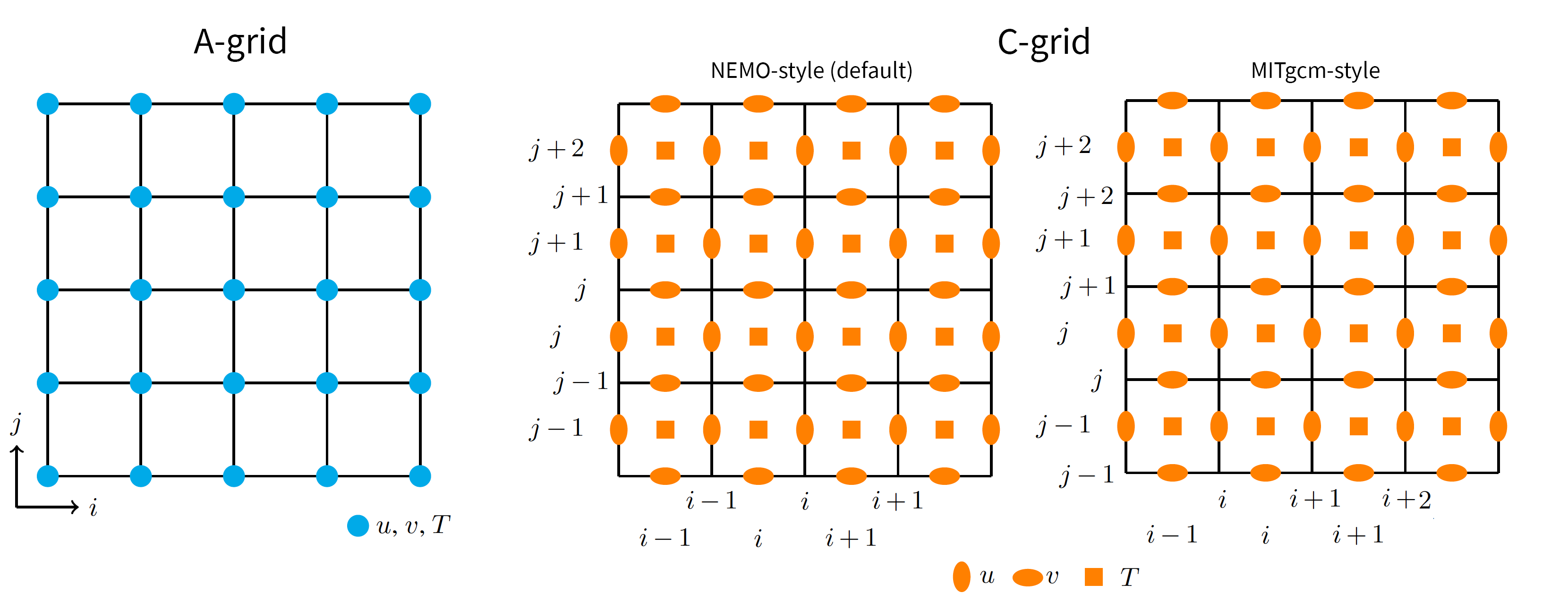
Note that different models use different indices to relate the location of the staggered velocities to the cell centers. The default C-grid indexing notation in Parcels is the same as for NEMO (middle panel): U[j, i] is located between the cell corners [j-1, i] and [j, i], and V[j, i] is located between cell corners [j, i-1] and [j, i].
Now, as you’ve noticed on the grid illustrated on the figure, there are 4x4 cells. The grid providing the cell corners is a 5x5 grid, but there are only 4x5 U nodes and 5x4 V nodes, since the grids are staggered. This implies that the first row of U data and the first column of V data is never used (and do not physically exist), but the U and V fields are correctly provided on a 5x5 table. If your original data are provided on a 4x5 U grid and a 5x4 V grid, you need to
regrid your table to follow Parcels notation before creating a FieldSet!
MITgcm uses a different indexing: U[j, i] is located between the cell corners [j, i] and [j+1, i], and V[j, i] is located between cell corners [j, i] and [j, i+1]. If you use xmitgcm to write your data to a NetCDF file, U and V will have the same dimensions as your grid (in the above case 4x4 rather than 5x5 as in NEMO), meaning that the last column of U and the last row of V are omitted. In MITgcm, these
either correspond to a solid boundary, or in the case of a periodic domain, to the first column and row respectively. In the latter case, and assuming your model domain is periodic, you can use the FieldSet.add_periodic_halo method to make sure particles can be correctly interpolated in the last zonal/meridional cells.
Parcels can take care of loading C-grid data for you, through the general FieldSet.from_c_grid_dataset method (which takes a gridindexingtype argument), and the model-specific methods FieldSet.from_nemo and FieldSet.from_mitgcm.
The only information that Parcels needs is the location of the 4 corners of the cell, which are called the \(f\)-node. Those are the ones provided by U.grid (and are equal to the ones in V.grid). Parcels does not need the exact location of the U and V nodes, because in C-grids, U and V nodes are always located in the same position relative to the \(f\)-node.
Importantly, the interpolation of velocities on Arakawa C-grids is done in barycentric coordinates: \(\xi\), \(\eta\) and \(\zeta\) instead of longitude, latitude and depth. These coordinates are always between 0 and 1, measured from the corner of the grid cell. This is more accurate than simple linear interpolation on curvilinear grids.
When calling FieldSet.from_c_grid_dataset() or a method that is based on it like FieldSet.from_nemo(), Parcels automatically sets the interpolation method for the U, V and W Fields to cgrid_velocity. With this interpolation method, the velocity interpolation follows the description in Section 2.1.2 of Delandmeter and Van Sebille (2019).
NEMO Example#
[1]:
import warnings
from glob import glob
from os import path

import numpy as np

import parcels
Let’s see how this works. We’ll use the NemoNorthSeaORCA025-N006_data data, which is on an Arakawa C-grid. If we create the FieldSet using the coordinates in the U, V and W files, we get an Error as seen below:
[2]:
example_dataset_folder = parcels.download_example_dataset(
    "NemoNorthSeaORCA025-N006_data"
)
ufiles = sorted(glob(f"{example_dataset_folder}/ORCA*U.nc"))
vfiles = sorted(glob(f"{example_dataset_folder}/ORCA*V.nc"))
wfiles = sorted(glob(f"{example_dataset_folder}/ORCA*W.nc"))

filenames = {"U": ufiles, "V": vfiles, "W": wfiles}
variables = {"U": "uo", "V": "vo", "W": "wo"}
dimensions = {
    "U": {
        "lon": "nav_lon",
        "lat": "nav_lat",
        "depth": "depthu",
        "time": "time_counter",
    },
    "V": {
        "lon": "nav_lon",
        "lat": "nav_lat",
        "depth": "depthv",
        "time": "time_counter",
    },
    "W": {
        "lon": "nav_lon",
        "lat": "nav_lat",
        "depth": "depthw",
        "time": "time_counter",
    },
}

fieldset = parcels.FieldSet.from_nemo(filenames, variables, dimensions)
---------------------------------------------------------------------------
ValueError                                Traceback (most recent call last)
/Users/erik/Codes/ParcelsCode/docs/examples/documentation_indexing.ipynb Cell 5 line 2
      <a href='vscode-notebook-cell:/Users/erik/Codes/ParcelsCode/docs/examples/documentation_indexing.ipynb#W4sZmlsZQ%3D%3D?line=6'>7</a> variables = {"U": "uo", "V": "vo", "W": "wo"}
      <a href='vscode-notebook-cell:/Users/erik/Codes/ParcelsCode/docs/examples/documentation_indexing.ipynb#W4sZmlsZQ%3D%3D?line=7'>8</a> dimensions = {
      <a href='vscode-notebook-cell:/Users/erik/Codes/ParcelsCode/docs/examples/documentation_indexing.ipynb#W4sZmlsZQ%3D%3D?line=8'>9</a>     "U": {
     <a href='vscode-notebook-cell:/Users/erik/Codes/ParcelsCode/docs/examples/documentation_indexing.ipynb#W4sZmlsZQ%3D%3D?line=9'>10</a>         "lon": "nav_lon",
   (...)
     <a href='vscode-notebook-cell:/Users/erik/Codes/ParcelsCode/docs/examples/documentation_indexing.ipynb#W4sZmlsZQ%3D%3D?line=25'>26</a>     },
     <a href='vscode-notebook-cell:/Users/erik/Codes/ParcelsCode/docs/examples/documentation_indexing.ipynb#W4sZmlsZQ%3D%3D?line=26'>27</a> }
---> <a href='vscode-notebook-cell:/Users/erik/Codes/ParcelsCode/docs/examples/documentation_indexing.ipynb#W4sZmlsZQ%3D%3D?line=28'>29</a> fieldset = FieldSet.from_nemo(filenames, variables, dimensions)

File ~/Codes/ParcelsCode/parcels/fieldset.py:545, in FieldSet.from_nemo(cls, filenames, variables, dimensions, indices, mesh, allow_time_extrapolation, time_periodic, tracer_interp_method, chunksize, **kwargs)
    543 if kwargs.pop('gridindexingtype', 'nemo') != 'nemo':
    544     raise ValueError("gridindexingtype must be 'nemo' in FieldSet.from_nemo(). Use FieldSet.from_c_grid_dataset otherwise")
--> 545 fieldset = cls.from_c_grid_dataset(filenames, variables, dimensions, mesh=mesh, indices=indices, time_periodic=time_periodic,
    546                                    allow_time_extrapolation=allow_time_extrapolation, tracer_interp_method=tracer_interp_method,
    547                                    chunksize=chunksize, gridindexingtype='nemo', **kwargs)
    548 if hasattr(fieldset, 'W'):
    549     fieldset.W.set_scaling_factor(-1.)

File ~/Codes/ParcelsCode/parcels/fieldset.py:656, in FieldSet.from_c_grid_dataset(cls, filenames, variables, dimensions, indices, mesh, allow_time_extrapolation, time_periodic, tracer_interp_method, gridindexingtype, chunksize, **kwargs)
    584 """Initialises FieldSet object from NetCDF files of Curvilinear NEMO fields.
    585
    586 See `here <../examples/documentation_indexing.ipynb>`__
   (...)
    653     Keyword arguments passed to the :func:`Fieldset.from_netcdf` constructor.
    654 """
    655 if 'U' in dimensions and 'V' in dimensions and dimensions['U'] != dimensions['V']:
--> 656     raise ValueError("On a C-grid, the dimensions of velocities should be the corners (f-points) of the cells, so the same for U and V. "
    657                      "See also ../examples/documentation_indexing.ipynb")
    658 if 'U' in dimensions and 'W' in dimensions and dimensions['U'] != dimensions['W']:
    659     raise ValueError("On a C-grid, the dimensions of velocities should be the corners (f-points) of the cells, so the same for U, V and W. "
    660                      "See also ../examples/documentation_indexing.ipynb")

ValueError: On a C-grid, the dimensions of velocities should be the corners (f-points) of the cells, so the same for U and V. See also ../examples/documentation_indexing.ipynb
We can still load the data this way, if we use the FieldSet.from_netcdf() method. But because this method assumes the data is on an Arakawa-A grid, this will mean wrong interpolation.
[3]:
fieldsetA = parcels.FieldSet.from_netcdf(filenames, variables, dimensions)
Instead, we need to provide the coordinates of the \(f\)-points. In NEMO, these are called glamf, gphif and depthw (in MITgcm, these would be called XG, YG and Zl). The first two are in the coordinates.nc file, the last one is in the W file.
[4]:
mesh_mask = f"{example_dataset_folder}/coordinates.nc"

filenames = {
    "U": {"lon": mesh_mask, "lat": mesh_mask, "depth": wfiles[0], "data": ufiles},
    "V": {"lon": mesh_mask, "lat": mesh_mask, "depth": wfiles[0], "data": vfiles},
    "W": {"lon": mesh_mask, "lat": mesh_mask, "depth": wfiles[0], "data": wfiles},
}

# Note that all variables need the same dimensions in a C-Grid
c_grid_dimensions = {
    "lon": "glamf",
    "lat": "gphif",
    "depth": "depthw",
    "time": "time_counter",
}
dimensions = {
    "U": c_grid_dimensions,
    "V": c_grid_dimensions,
    "W": c_grid_dimensions,
}

with warnings.catch_warnings():
    warnings.simplefilter("ignore", parcels.FileWarning)
    fieldsetC = parcels.FieldSet.from_nemo(filenames, variables, dimensions)
Note by the way, that we used warnings.catch_warnings() with warnings.simplefilter("ignore", parcels.FileWarning) to wrap the FieldSet.from_nemo() call above. This is to silence an expected warning because the time dimension in the coordinates.nc file can’t be decoded by xarray.
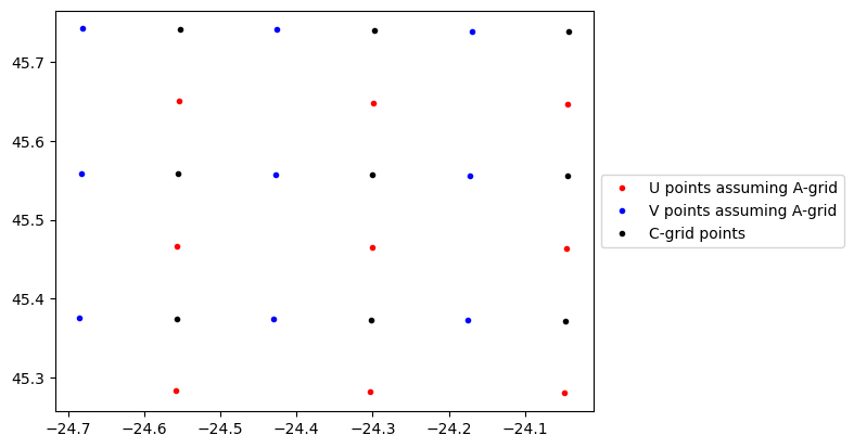
We can plot the different grid points to see that indeed, the longitude and latitude of fieldsetA.U and fieldsetA.V are different.
[5]:
import matplotlib.pyplot as plt
from mpl_toolkits.mplot3d import Axes3D  # noqa

fig, ax = plt.subplots()
nind = 3
ax1 = ax.plot(
    fieldsetA.U.grid.lon[:nind, :nind],
    fieldsetA.U.grid.lat[:nind, :nind],
    ".r",
    label="U points assuming A-grid",
)
ax2 = ax.plot(
    fieldsetA.V.grid.lon[:nind, :nind],
    fieldsetA.V.grid.lat[:nind, :nind],
    ".b",
    label="V points assuming A-grid",
)

ax3 = ax.plot(
    fieldsetC.U.grid.lon[:nind, :nind],
    fieldsetC.U.grid.lat[:nind, :nind],
    ".k",
    label="C-grid points",
)

ax.legend(handles=[ax1[0], ax2[0], ax3[0]], loc="center left", bbox_to_anchor=(1, 0.5))
plt.show()
Further information about the NEMO C-grids is available in the NEMO 3D tutorial.
Arakawa B-grids#
Interpolation for Arakawa B-grids is detailed in Section 2.1.3 of Delandmeter and Van Sebille (2019). Again, the dimensions that need to be provided are those of the barycentric cell edges (i, j, k).
To load B-grid data, you can use the method FieldSet.from_b_grid_dataset, or specifically in the case of POP-model data FieldSet.from_pop.
3D C- and B-grids#
For 3D C-grids and B-grids, the idea is the same. It is important to follow the indexing notation, which is defined in Parcels and in Delandmeter and Van Sebille (2019). In 3D C-grids, the vertical (W) velocities are at the top and bottom. Note that in the vertical, the bottom velocity is often omitted, since a no-flux boundary conditions implies a zero vertical velocity at the ocean floor. That means that the vertical
dimension of W often corresponds to the amount of vertical levels.