Diffusion#
In Eulerian ocean models, sub-grid scale dispersion of tracers such as heat, salt, or nutrients is often parameterized as a diffusive process. In Lagrangian particle simulations, sub-grid scale effects can be parameterized as a stochastic process, randomly displacing a particle position in proportion to the local eddy diffusivity (Van Sebille et al. 2018). Parameterizing sub-grid scale dispersion may be especially important when coarse velocity fields are used that do not resolve mesoscale eddies (Shah et al., 2017). This tutorial explains how to use a sub-grid scale parameterization in Parcels that is consistent with the advection-diffusion equation used in Eulerian models.
Stochastic differential equations (SDE) consistent with advection-diffusion#
The time-evolution of a stochastic process is described by a stochastic differential equation. The time-evolution of the conditional probability density of a stochastic process is described by a Fokker-Planck equation (FPE). The advection-diffusion equation, describing the evolution of a tracer, can be written as a Fokker-Planck equation. Therefore, we can formulate a stochastic differential equation for a particle in the Lagrangian frame undergoing advection with stochastic noise proportional to the local diffusivity in a way that is consistent with advection-diffusion in the Eulerian frame. For details, see Shah et al., 2011 and van Sebille et al., 2018.
The stochastic differential equation for a particle trajectory including diffusion is
where \(\mathbf{X}\) is the particle position vector (\(\mathbf{x}_0\) being the initial position vector), and \(\mathbf{u}\) the velocity vector. \(\mathbf{V}\) is calculated from the diffusivity tensor \(\mathbf{K} = \frac{1}{2} \mathbf{V} \cdot \mathbf{V}^T\) and \(d\mathbf{W}(t)\) a Wiener increment (normally distributed with zero mean and variance \(dt\)). Particle distributions obtained by solving the above equation are therefore consistent with Eulerian concentrations found by solving the advection-diffusion equation.
In three-dimensional ocean models diffusion operates along slopes of neutral buoyancy. To account for these slopes, the 3D diffusivity tensor \(\mathbf{K}\) (and therefore \(\mathbf{V}\)) contains off-diagonal components. Three-dimensional advection-diffusion is not yet implemented in Parcels, but it is currently under development. Here we instead focus on the simpler case of diffusion in a horizontal plane, where diffusivity is specified only in the zonal and meridional direction, i.e.
The above stochastic differential equation then becomes
where \(a_i = v_i + \partial_i K_i(x, y)\) is the deterministic drift term and \(b_i = \sqrt{2K_i(x, y)}\) a stochastic noise term (\(\partial_i\) denotes the partial derivative with respect to \(i\)).
Numerical Approximations of SDEs#
The simplest numerical approximation of the above SDEs is obtained by replacing \(dt\) by a finite time discrete step \(\Delta t\) and \(dW\) by a discrete increment \(\Delta W\), yielding the Euler-Maruyama (EM) scheme (Maruyama, 1955):
with a similar expression for \(Y\).
A higher-order scheme is found by including extra terms from a Taylor expansion on our SDE, yielding the Milstein scheme of order 1 (M1):
which can be rewritten by explicitly writing \(b_x\partial_x b_x\) as \(\partial_x K_x(z)\):
The extra term in the M1 scheme provides extra accuracy at negligible computational cost.
The spatial derivatives in the EM and M1 schemes can be approximated by a central difference. Higher order numerical schemes (see Gräwe et al., 2012) include higher order derivatives. Since Parcels uses bilinear interpolation, these higher order derivatives cannot be computed, meaning that higher order numerical schemes cannot be used.
An overview of numerical approximations for SDEs in a particle tracking setting can be found in Gräwe (2011).
Using Advection-Diffusion Kernels in Parcels#
The EM and M1 advection-diffusion approximations are available as AdvectionDiffusionEM and AdvectionDiffusionM1, respectively. The AdvectionDiffusionM1 kernel should be the default choice, as the increased accuracy comes at negligible computational cost.
The advection component of these kernels is similar to that of the Explicit Euler advection kernel (AdvectionEE). In the special case where diffusivity is constant over the entire domain, the diffusion-only kernel DiffusionUniformKh can be used in combination with an advection kernel of choice. Since the diffusivity here is space-independent, gradients are not calculated, increasing efficiency. The diffusion-step can in this case be computed after or before advection, thus allowing you
to chain kernels using the + operator.
Just like velocities, diffusivities are passed to Parcels in the form of Field objects. When using DiffusionUniformKh, they should be added to the FieldSet object as constant fields, e.g. fieldset.add_constant_field("Kh_zonal", 1, mesh="flat").
To make a central difference approximation for computing the gradient in diffusivity, a resolution for this approximation dres is needed: Parcels approximates the gradients in diffusivities by using their values at the particle’s location ± dres (in both \(x\) and \(y\)). A value of dres must be specified and added to the FieldSet by the user (e.g. fieldset.add_constant("dres", 0.01)). Currently, it is unclear what the best value of dres is. From experience, its
size of dres should be smaller than the spatial resolution of the data, but within reasonable limits of machine precision to avoid numerical errors. We are working on a method to compute gradients differently so that specifying dres is not necessary anymore.
Example: Impermeable Diffusivity Profile#
Let’s see the AdvectionDiffusionM1 in action and see why it’s preferable over the AdvectionDiffusionEM kernel. To do so, we create an idealized profile with diffusivities \(K_\text{zonal}\) uniform everywhere (\(K_\text{zonal} = \bar{K}=0.5\)) and \(K_\text{meridional}\) constant in the zonal direction, while having the following profile in the meridional direction:
with \(L\) being the basin length scale, \(\alpha\) as a parameter determining the steepness in the gradient in the profile. This profile is similar to that used by Gräwe (2011), now used in the meridional direction for illustrative purposes.
Let’s plot \(K_\text{meridional}(y)\):
[1]:
from datetime import timedelta

import matplotlib.pyplot as plt
import numpy as np
import trajan as ta
import xarray as xr

import parcels
[2]:
K_bar = 0.5  # Average diffusivity
alpha = 1.0  # Profile steepness
L = 1.0  # Basin scale

# Number of grid cells in y_direction (101 +2)
# one level above and one below, where fields are set to zero
Ny = 103

# Spatial resolution
dy = 1.03 / Ny

# y-coordinates for grid
y = np.linspace(-0.01, 1.01, 103)

# y-coordinates used for setting diffusivity
y_K = np.linspace(0.0, 1.0, 101)

# Placeholder for fraction term in K(y) formula
beta = np.zeros(y_K.shape)

for yi in range(len(y_K)):
    if y_K[yi] < L / 2:
        beta[yi] = y_K[yi] * np.power(L - 2 * y_K[yi], 1 / alpha)
    elif y_K[yi] >= L / 2:
        beta[yi] = (L - y_K[yi]) * np.power(2 * y_K[yi] - L, 1 / alpha)
Kh_meridional = (
    0.1
    * (2 * (1 + alpha) * (1 + 2 * alpha))
    / (alpha**2 * np.power(L, 1 + 1 / alpha))
    * beta
)
Kh_meridional = np.concatenate((np.array([0]), Kh_meridional, np.array([0])))
[3]:
plt.plot(Kh_meridional, y)
plt.ylabel("y")
plt.xlabel(r"$K_{meridional}$")
plt.show()
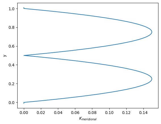
In this profile, diffusivity drops to 0 at \(y=0.5\) and at \(y=0\) and \(y=1\). In the absence of advection, particles starting out in one half of the domain should remain confined to that half as they are unable to cross the points where the diffusivity drops to 0. The line \(y=0.5\) should therefore provide an impermeable barrier.
Now we can put this idealized profile into a flat fieldset:
[4]:
xdim, ydim = (1, Ny)
data = {
    "U": np.zeros(ydim),
    "V": np.zeros(ydim),
    "Kh_zonal": K_bar * np.ones(ydim),
    "Kh_meridional": Kh_meridional,
}
dims = {"lon": 1, "lat": np.linspace(-0.01, 1.01, ydim, dtype=np.float32)}
fieldset = parcels.FieldSet.from_data(
    data, dims, mesh="flat", allow_time_extrapolation=True
)
fieldset.add_constant("dres", 0.00005)
We release 100 particles at (\(x=0\), \(y=0.75\)).
[5]:
def get_test_particles():
    return parcels.ParticleSet.from_list(
        fieldset,
        pclass=parcels.JITParticle,
        lon=np.zeros(100),
        lat=np.ones(100) * 0.75,
        time=np.zeros(100),
        lonlatdepth_dtype=np.float64,
    )
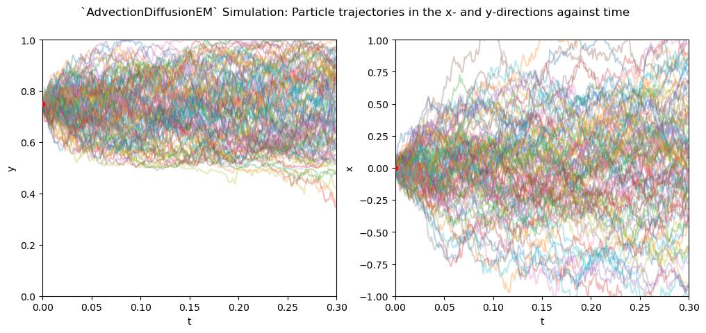
Now we will simulate the advection and diffusion of the particles using the AdvectionDiffusionM1 kernel. We run the simulation for 0.3 seconds, with a numerical timestep \(\Delta t = 0.001\)s. We also write away particle locations at each timestep for plotting. Note that this will hinder a runtime comparison between kernels, since it will cause most time to be spent on I/O.
[6]:
dt = 0.001
testParticles = get_test_particles()
output_file = testParticles.ParticleFile(
    name="M1_out.zarr", chunks=(len(testParticles), 50), outputdt=timedelta(seconds=dt)
)

parcels.ParcelsRandom.seed(1636)  # Random seed for reproducibility

testParticles.execute(
    parcels.AdvectionDiffusionM1,
    runtime=timedelta(seconds=0.3),
    dt=timedelta(seconds=dt),
    output_file=output_file,
)
INFO: Compiled ParcelsRandom ==> /var/folders/1n/500ln6w97859_nqq86vwpl000000gr/T/parcels-504/parcels_random_4217ba4c-0bce-4de3-8bfc-a59aaf457cca.c
INFO: Output files are stored in M1_out.zarr.
100%|██████████| 0.3/0.3 [00:01<00:00,  5.11s/it]
[7]:
M1_out = xr.open_zarr("M1_out.zarr")
We can plot the individual coordinates of the particle trajectories against time (\(x\) against \(t\) and \(y\) against \(t\)) to investigate how diffusion works along each axis.
[8]:
fig, ax = plt.subplots(1, 2)
fig.set_figwidth(12)

x = np.arange(0, 0.3, 0.001)
for data, ai, dim, ystart, ylim in zip(
    [M1_out.lat, M1_out.lon], ax, ("y", "x"), (0.75, 0), [(0, 1), (-1, 1)]
):
    ai.plot(x, data.T[: len(x), :], alpha=0.3)
    ai.scatter(0, ystart, s=20, c="r", zorder=3)
    ai.set_xlabel("t")
    ai.set_ylabel(dim)
    ai.set_xlim(0, 0.3)
    ai.set_ylim(ylim)

fig.suptitle(
    "`AdvectionDiffusionM1` Simulation: "
    f"Particle trajectories in the x- and y-directions against time"
)
plt.show()

We see that the along the meridional direction, particles remain confined to the ‘upper’ part of the domain, not crossing the impermeable barrier where the diffusivity drops to zero. In the zonal direction, particles follow random walks, since all terms involving gradients of the diffusivity are zero.
Now let’s execute the simulation with the AdvectionDiffusionEM kernel instead.
[9]:
dt = 0.001
testParticles = get_test_particles()
output_file = testParticles.ParticleFile(
    name="EM_out.zarr", chunks=(len(testParticles), 50), outputdt=timedelta(seconds=dt)
)
parcels.ParcelsRandom.seed(1636)  # Random seed for reproducibility
testParticles.execute(
    parcels.AdvectionDiffusionEM,
    runtime=timedelta(seconds=0.3),
    dt=timedelta(seconds=dt),
    output_file=output_file,
)
INFO: Output files are stored in EM_out.zarr.
100%|██████████| 0.3/0.3 [00:01<00:00,  5.10s/it]
[10]:
EM_out = xr.open_zarr("EM_out.zarr")
[11]:
fig, ax = plt.subplots(1, 2)
fig.set_figwidth(12)

x = np.arange(0, 0.3, 0.001)
for data, ai, dim, ystart, ylim in zip(
    [EM_out.lat, EM_out.lon], ax, ("y", "x"), (0.75, 0), [(0, 1), (-1, 1)]
):
    ai.plot(x, data.T[: len(x), :], alpha=0.3)
    ai.scatter(0, ystart, s=20, c="r", zorder=3)
    ai.set_xlabel("t")
    ai.set_ylabel(dim)
    ai.set_xlim(0, 0.3)
    ai.set_ylim(ylim)

fig.suptitle(
    "`AdvectionDiffusionEM` Simulation: "
    f"Particle trajectories in the x- and y-directions against time"
)
plt.show()
The Wiener increments for both simulations are equal, as they are fixed through a random seed. As we can see, the Euler-Maruyama scheme performs worse than the Milstein scheme, letting particles cross the impermeable barrier at \(y=0.5\). In contrast, along the zonal direction, particles follow the same random walk as in the Milstein scheme, which is expected since the extra terms in the Milstein scheme are zero in this case.
Example: Using horizontal diffusion calculated from velocity fields#
In the case when velocity fields are available, there is the possibility to calculate coefficients of diffusion based on closure parameterizations. The Smagorinsky method (Smagorinsky, 1963), which was originally proposed as a parameterization for horizontal eddy viscosity, is often used to parameterize horizontal eddy diffusivity as well. It computes the eddy diffusivity as
where \(C_s\), the Smagorinsky constant, is a dimensionless tuning parameter. It uses the grid area \(\Delta x \Delta y\) as its spatial scale, and the norm of the strain rate tensor as its time scale, given as the square-rooted term.
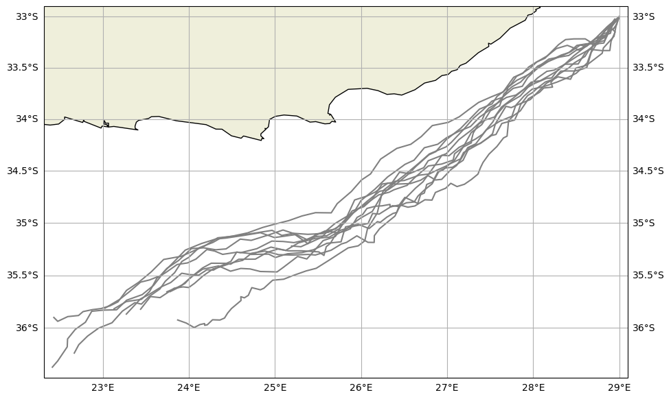
Let’s see the example of implementation of the Smagorinsky method to the GlobalCurrents files of the region around South Africa. For simplicity, we are not taking gradients in the Smagorinsky-computed diffusivity field into account here.
First, create a new kernel for Smagorinsky diffusion method:
[12]:
def smagdiff(particle, fieldset, time):
    dx = 0.01
    # gradients are computed by using a local central difference.
    updx, vpdx = fieldset.UV[time, particle.depth, particle.lat, particle.lon + dx]
    umdx, vmdx = fieldset.UV[time, particle.depth, particle.lat, particle.lon - dx]
    updy, vpdy = fieldset.UV[time, particle.depth, particle.lat + dx, particle.lon]
    umdy, vmdy = fieldset.UV[time, particle.depth, particle.lat - dx, particle.lon]

    dudx = (updx - umdx) / (2 * dx)
    dudy = (updy - umdy) / (2 * dx)

    dvdx = (vpdx - vmdx) / (2 * dx)
    dvdy = (vpdy - vmdy) / (2 * dx)

    A = fieldset.cell_areas[time, 0, particle.lat, particle.lon]
    sq_deg_to_sq_m = (1852 * 60) ** 2 * math.cos(particle.lat * math.pi / 180)
    A = A / sq_deg_to_sq_m
    Kh = fieldset.Cs * A * math.sqrt(dudx**2 + 0.5 * (dudy + dvdx) ** 2 + dvdy**2)

    dlat = parcels.ParcelsRandom.normalvariate(0.0, 1.0) * math.sqrt(
        2 * math.fabs(particle.dt) * Kh
    )
    dlon = parcels.ParcelsRandom.normalvariate(0.0, 1.0) * math.sqrt(
        2 * math.fabs(particle.dt) * Kh
    )

    particle_dlat += dlat
    particle_dlon += dlon
Reading velocity fields from netcdf files
[13]:
example_dataset_folder = parcels.download_example_dataset("GlobCurrent_example_data")
filenames = {
    "U": f"{example_dataset_folder}/20*.nc",
    "V": f"{example_dataset_folder}/20*.nc",
}
variables = {
    "U": "eastward_eulerian_current_velocity",
    "V": "northward_eulerian_current_velocity",
}
dimensions = {"lat": "lat", "lon": "lon", "time": "time"}

fieldset = parcels.FieldSet.from_netcdf(filenames, variables, dimensions)
Adding parameters (cell_areas – areas of computational cells, and Cs – Smagorinsky constant) to fieldset that are needed for the smagdiff kernel
[14]:
x = fieldset.U.grid.lon
y = fieldset.U.grid.lat

cell_areas = parcels.Field(
    name="cell_areas", data=fieldset.U.cell_areas(), lon=x, lat=y
)
fieldset.add_field(cell_areas)

fieldset.add_constant("Cs", 0.1)
In the example, particles are released at one location periodically (every hour) for 12 hours
[15]:
time = np.arange(0, 43200, 3600)
lon = [29] * len(time)
lat = [-33] * len(time)
pset = parcels.ParticleSet(
    fieldset=fieldset, pclass=parcels.JITParticle, lon=lon, lat=lat, time=time
)
Simulating the particles moving during 7 days using advection (AdvectionRK4) and diffusion (smagdiff) kernels.
[16]:
def DeleteParticle(particle, fieldset, time):
    if particle.state == parcels.StatusCode.ErrorOutOfBounds:
        particle.delete()


output_file = pset.ParticleFile(
    name="Global_smagdiff.zarr", outputdt=timedelta(hours=3), chunks=(1, 57)
)

parcels.ParcelsRandom.seed(1636)  # Random seed for reproducibility

pset.execute(
    [parcels.AdvectionRK4, smagdiff, DeleteParticle],
    runtime=timedelta(days=7),
    dt=timedelta(minutes=5),
    output_file=output_file,
)
INFO: Output files are stored in Global_smagdiff.zarr.
100%|██████████| 604800.0/604800.0 [00:02<00:00, 222140.27it/s]
Visualize the trajectories using the trajan package
[17]:
ds = xr.open_zarr("Global_smagdiff.zarr")

ds.traj.plot()
plt.show()
References#
Gräwe, U. (2011). “Implementation of high-order particle-tracking schemes in a water column model.” Ocean Modelling, 36(1), 80–89. https://doi.org/10.1016/j.ocemod.2010.10.002
Gräwe, Deleersnijder, Shah & Heemink (2012). “Why the Euler scheme in particle tracking is not enough: The shallow-sea pycnocline test case.” Ocean Dynamics, 62(4), 501–514. https://doi.org/10.1007/s10236-012-0523-y
Maruyama, G. (1955). “Continuous Markov processes and stochastic equations.” Rendiconti del Circolo Matematico di Palermo, 4(1), 48.
van Sebille et al. (2018). “Lagrangian ocean analysis: Fundamentals and practices.” Ocean Modelling, 121, 49–75. https://doi.org/10.1016/j.ocemod.2017.11.008
Shah, S. H. A. M., Heemink, A. W., & Deleersnijder, E. (2011). “Assessing Lagrangian schemes for simulating diffusion on non-flat isopycnal surfaces.” Ocean Modelling, 39(3–4), 351–361. https://doi.org/10.1016/j.ocemod.2011.05.008 https://doi.org/10.1016/j.ocemod.2011.05.008
Shah, Primeau, Deleersnijder & Heemink (2017). “Tracing the Ventilation Pathways of the Deep North Pacific Ocean Using Lagrangian Particles and Eulerian Tracers.” Journal of Physical Oceanography, 47(6), 1261–1280. https://doi.org/10.1175/JPO-D-16-0098.1
Smagorinsky, J. (1963). “General circulation experiments with primitive equations. 1. The basic experiment.” Monthly Weather Review, 91, 99–164. https://doi.org/10.1175/1520-0493(1963)091%3C0099:GCEWTP%3E2.3.CO;2