Parcels trajectories with geospatial data types and software#
Shapefile
Geopackage
GeoJSON
KML
This allows for easy integration of Parcels output with any geospatial workflows you have, or geospatial tools you would like for further visualization and analysis. Geospatial software covered in this tutorial include:
This code has been written to make it as “production ready” and “copy pastable” as possible to help with your workflows. This tutorial also highlights the limitations of some geospatial datasets and tools when it comes to working with large datasets (which parcels tends to output).
This tutorial requires the following packages:
geopandas to create the geospatial datasets (
conda install -c conda-forge geopandas)lxml to create KML files for Google Earth (
conda install lxml)
This tutorial saves all generated data output in a folder tutorial_geospatial_output to avoid clogging the working directory. If you’re re-running this notebook, be sure to delete this folder so that the notebook doesn’t encounter writing issues.
GIS data types#
There are mainly two types of geospatial data:
Raster data
Vector data
See this article for an explainer of raster vs vector data types.
Various geospatial dataset types exist for raster and vector data. Here we go over a few of them, discussing their advantages and disadvantages.
NetCDF (.nc)#
A raster data format for storing and sharing large, multi-dimensional arrays of scientific data, often used for gridded climate and oceanographic datasets. May need some processing before visualizing depending on setup of the NetCDF.
Shapefile (.shp, …)#
The longest standing geospatial vector data format used for storing location data and associated attribute information. Shapefile is a multifile format, where the dataset is split into files with different extensions handling vector (.shp), indexing (.shx), attribute (.dbf), encoding (.cpg), and projection (.prj) information. The shapefile is a geospatial data format with many limitations compared to other geospatial data formats.
Pros:
The oldest data format. Has wide adoption across various GIS tools.
Cons:
Limits on:
variable name lengths (10 characters)
variable types
file size (2Gb max)
No NULL value
No time data type.
Can only contain a single layer (i.e. you can’t mix geospatial data types in a single file).
GeoJSON (.geojson)#
A lightweight, human-readable, vector data format for encoding geospatial data structures, such as points, lines, and polygons, using JavaScript Object Notation (JSON). Commonly used in web applications.
KML (.kml) and KMZ (.kmz)#
XML-based vector formats for expressing geographic annotations and visualizations on 2D maps and 3D Earth browsers, such as Google Earth. KMZ is a compressed version of KML.
GeoPackage (.gpkg)#
A modern, open, standards-based, platform-independent format for storing geospatial data. Operates using an SQLite database, and is capable of storing multiple layers in a single dataset. Can contain raster and vector layers.
Geodatabase (.gdb)#
A proprietary Esri format for storing, querying, and managing geospatial data, including vector, raster, and tabular data. This tutorial does not cover Geodatabases.
For geospatial vector datasets, layers can only contain one feature type. Each feature in a geospatial dataset can have associated data (timestamps, text, numeric values) depending on what the data represents. There are 3 types of features in geospatial datasets:
Point: Describes individual coordinates on earth.
Linestring: Describes individual lines on earth (is composed of a sequence of coordinates, which are joined in an open loop).
Polygon: Describes individual polygons on earth (is composed of a sequence of coordinates, which are joined in a closed loop).
Here there are two logical choices for representing particle trajectory data, using points or linestrings. Using points, all the data (including timestamps) is preserved, but the path of the particle may not be inherently evident on the software being used to load the point data. The timestamp information is tied as data for that point, and may not be visualized by the software. Representing trajectories as linestrings makes it easy to visualize trajectories in GIS software, but extra data regarding the individual point observations (i.e. all data except (lon, lat) location data) is lost in this format.
These limitations mainly apply to Shapefile, GeoJSON, GeoPackage, and Geodatabase formats when used in GIS applications. As explored later, Google Earth (KML) has syntax specifically for visualizing trajectories, and Kepler accepts modified GeoJSON to represent trajectory data.
Creating geospatial datasets from parcels output#
First, we run import all the packages needed for this tutorial, run an example parcels simulation and save the output.
[1]:
import datetime
import json
from datetime import timedelta
from pathlib import Path

import geopandas as gpd
import numpy as np
import requests
import xarray as xr
from lxml import etree
from shapely.geometry import LineString, Point

import parcels

DATA_OUTPUT_FOLDER = Path("tutorial_geospatial_output")
DATA_OUTPUT_FOLDER.mkdir(exist_ok=True)
DATA_OUTPUT_NAME = "agulhas_trajectories"
[2]:
# An example parcels simulation
data_folder = parcels.download_example_dataset("GlobCurrent_example_data")
filenames = filename = str(data_folder / "20*.nc")
variables = {
    "U": "eastward_eulerian_current_velocity",
    "V": "northward_eulerian_current_velocity",
}
dimensions = {
    "lat": "lat",
    "lon": "lon",
    "time": "time",
}

fieldset = parcels.FieldSet.from_netcdf(filenames, variables, dimensions)

# Mesh of particles
lons, lats = np.meshgrid(range(15, 35, 2), range(-40, -30, 2))
pset = parcels.ParticleSet(
    fieldset=fieldset, pclass=parcels.JITParticle, lon=lons, lat=lats
)
dt = timedelta(hours=24)
output_file = pset.ParticleFile(
    name=DATA_OUTPUT_FOLDER / f"{DATA_OUTPUT_NAME}.zarr", outputdt=dt
)


def DeleteParticle(particle, fieldset, time):
    if particle.state > 4:
        particle.delete()


pset.execute(
    [parcels.AdvectionRK4, DeleteParticle],
    runtime=timedelta(days=120),
    dt=dt,
    output_file=output_file,
)
INFO: Output files are stored in tutorial_geospatial_output/agulhas_trajectories.zarr.
100%|██████████| 10368000.0/10368000.0 [00:15<00:00, 651613.20it/s]
Now we have a zarr dataset stored in the tutorial_geospatial_example_trajectories.zarr folder. We can open this using xarray into an xarray.Dataset object and process it into different geospatial datasets.
First up is the easiest, NetCDF.
[3]:
ds_parcels = xr.open_zarr(DATA_OUTPUT_FOLDER / f"{DATA_OUTPUT_NAME}.zarr")

ds_parcels.to_netcdf(DATA_OUTPUT_FOLDER / f"{DATA_OUTPUT_NAME}.nc")
As the NetCDF format is very similar to zarr, there is no need for extra processing. The other datatypes will require some more work to convert the raster data to a vector format.
For this, geopandas is used which extends the pandas DataFrame object with various geospatial capabilities to create a GeoDataFrame object (learn more about the geopandas project). Geopandas, like pandas, operates with data in-memory, which will require the data to be loaded into RAM (as opposed to being lazy loaded like with NetCDF and zarr datasets). To avoid loading in huge datasets, we code in some safeguards. If your dataset is too large, it is
recommended you subset your xr.Dataset to reduce its size before proceeding with converting to the geospatial datasets.
[4]:
def parcels_to_geopandas(ds, suppress_warnings=False):
    """
    Converts your parcels data to a geopandas dataframe containing a point for
    every observation in the dataframe. Custom particle variables come along
    for the ride during the transformation. Any undefined observations are removed
    (correspond to the particle being deleted, or not having entered the simulation).

    Assumes your parcel output is in lat and lon.

    Parameters
    ----------
    ds : xr.Dataset
        Dataset object in the format of parcels output.

    suppress_warnings : bool
        Whether to ignore RAM warning.

    Returns
    -------
    geopandas.GeoDataFrame
        GeoDataFrame with point data for each particle observation in the dataset.
    """
    RAM_LIMIT_BYTES = 4 * 1000 * 1000  # 4 GB RAM limit

    if ds.nbytes > RAM_LIMIT_BYTES and not suppress_warnings:
        raise MemoryError(
            f"Dataset is {ds.nbytes:_} bytes, but RAM_LIMIT_BYTES set max to be {RAM_LIMIT_BYTES:_}."
        )

    df = (
        ds.to_dataframe().reset_index()  # Convert `obs` and `trajectory` indices to be columns instead
    )

    gdf = (
        gpd.GeoDataFrame(df, geometry=gpd.points_from_xy(df["lon"], df["lat"]))
        .drop(
            ["lon", "lat"], axis=1
        )  # No need for lon and lat cols. Included in geometry attribute
        .set_crs(
            "EPSG:4326"
        )  # Set coordinate reference system to EPSG:4326 (aka. WGS84; the lat lon reference system)
    )

    # Remove observations with no time from gdf (indicate particle has been removed, or isn't in simulation)
    invalid_observations = gdf["time"].isna()
    return gdf[~invalid_observations]


gdf_parcels = parcels_to_geopandas(ds_parcels)
gdf_parcels
[4]:
| trajectory | obs | time | z | geometry | |
|---|---|---|---|---|---|
| 0 | 0 | 0 | 2002-01-01 | 0.0 | POINT (15.00000 -40.00000) |
| 1 | 0 | 1 | 2002-01-02 | 0.0 | POINT (15.23998 -39.85211) |
| 2 | 0 | 2 | 2002-01-03 | 0.0 | POINT (15.55334 -39.81898) |
| 3 | 0 | 3 | 2002-01-04 | 0.0 | POINT (15.93826 -39.85509) |
| 4 | 0 | 4 | 2002-01-05 | 0.0 | POINT (16.46919 -39.67649) |
| ... | ... | ... | ... | ... | ... |
| 5932 | 49 | 3 | 2002-01-04 | 0.0 | POINT (33.59146 -32.07283) |
| 5933 | 49 | 4 | 2002-01-05 | 0.0 | POINT (33.81222 -32.14541) |
| 5934 | 49 | 5 | 2002-01-06 | 0.0 | POINT (34.14362 -32.15410) |
| 5935 | 49 | 6 | 2002-01-07 | 0.0 | POINT (34.57761 -32.23006) |
| 5936 | 49 | 7 | 2002-01-07 | 0.0 | POINT (34.57761 -32.23006) |
2562 rows × 5 columns
[5]:
# Output GeoDataFrame to geospatial file format (format inferred from extension)
gdf_parcels.to_file(DATA_OUTPUT_FOLDER / f"{DATA_OUTPUT_NAME}.geojson")
gdf_parcels.to_file(DATA_OUTPUT_FOLDER / f"{DATA_OUTPUT_NAME}.gpkg")

# Shapefile can't handle datetime objects. Converting to seconds since 01/01/1970.
gdf_shapefile = gdf_parcels.copy()
gdf_shapefile["time"] = (
    gdf_shapefile["time"] - datetime.datetime(1970, 1, 1)
).dt.total_seconds()
gdf_shapefile.to_file(
    DATA_OUTPUT_FOLDER / f"{DATA_OUTPUT_NAME}_shapefile"
)  # Saves in dedicated subfolder all shapefile component files

# Converting to KML is covered in the Google Earth software section
Now we have our observation data in vector format as individual points, lets create linestring objects for each trajectory. We then load in both geopackage files (point data, and trajectory linestrings) into QGIS for visualization.
[6]:
# Creating linestring objects
linestrings = [
    # trajectory_idx, linestring
]
for trajectory_idx, trajectory_gdf in gdf_parcels.groupby("trajectory"):
    trajectory_gdf = trajectory_gdf.sort_values("obs")
    points = trajectory_gdf["geometry"]
    if points.shape[0] == 1:
        continue  # Can't create LineString with one point
    linestring = LineString()
    linestrings.append((trajectory_idx, linestring))

gdf_parcels_linestring = gpd.GeoDataFrame(
    linestrings, columns=["trajectory", "geometry"]
)

# Save linestrings to geospatial dataset using the same commands as before
# E.g. geopackage
gdf_parcels_linestring.to_file(
    DATA_OUTPUT_FOLDER / f"{DATA_OUTPUT_NAME}_linestring.gpkg"
)
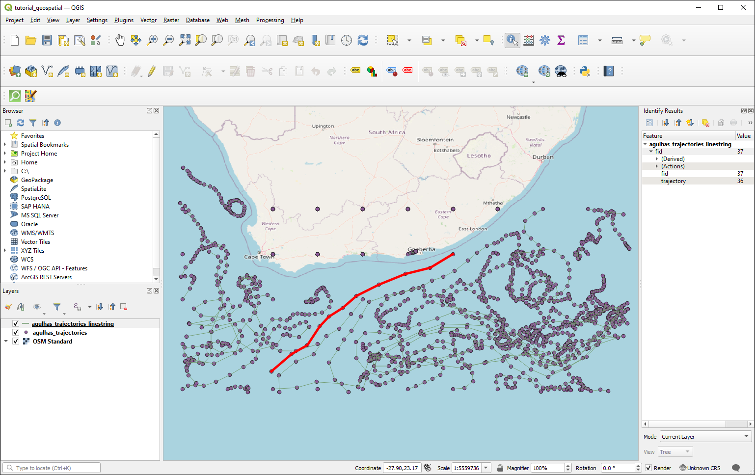
Geopandas is extremely versatile as a tool to explore and analyze geospatial data. The usefulness of geopandas when it comes to analysing parcels output is further explored in the example at the end of this tutorial.
Google Earth#
Here we convert the trajectories to KML using gx:Track objects (which can have time encoded in the trajectory). We use lxml, a general purpose XML data editor. fastkml is a good option for creating KML files, but in this case doesn’t explicitly support gx objects in its API. KMZ is just a compressed version of KML, and is not covered here.
[7]:
def parcels_geopandas_to_kml(
    gdf: gpd.GeoDataFrame,
    path,
    document_name="Parcels Particle Trajectories",
    rubber_ducks=True,
):
    """Writes parcels trajectories to KML file.

    Converts the GeoDataFrame from the `parcels_to_geopandas` function into KML
    for use in Google Earth. Each particle trajectory is converted to a gx:Track item
    to include timestamp information in the path.

    Only uses the trajectory ID, time, lon, and lat variables.

    Parameters
    ----------
    gdf : gpd.GeoDataFrame
        GeoDataFrame as output from the `parcels_to_geopandas` function

    path : pathlike
        Path to save the KML to.

    rubber_ducks : bool
        Replace default particle marker with rubber duck icon.


    See also
    --------
    More on gx:Track in KML:
    https://developers.google.com/kml/documentation/kmlreference#gx:track
    """
    # Define namspaces
    kml_ns = "http://www.opengis.net/kml/2.2"
    gx_ns = "http://www.google.com/kml/ext/2.2"

    kml_out = etree.Element("{%s}kml" % kml_ns, nsmap={None: kml_ns, "gx": gx_ns})
    document = etree.SubElement(
        kml_out, "Document", id="1", name="Particle trajectories"
    )

    # Custom icon styling
    if rubber_ducks:
        icon_styling = etree.fromstring(
            f"""<Style id="iconStyle">
                  <IconStyle>
                    <scale>0.8</scale>
                    <Icon>
                      <href>https://icons.iconarchive.com/icons/thesquid.ink/free-flat-sample/256/rubber-duck-icon.png</href>
                    </Icon>
                  </IconStyle>
                </Style>
            """
        )
        document.append(icon_styling)

    # Generating gx:Track items
    for trajectory_idx, trajectory_gdf in gdf.groupby("trajectory"):
        trajectory_gdf = trajectory_gdf.sort_values("obs")

        placemark = etree.SubElement(document, "Placemark")
        name_element = etree.SubElement(placemark, "name")
        name_element.text = str(trajectory_idx)

        # Link custom icon styling
        if rubber_ducks:
            style_url = etree.SubElement(placemark, "styleUrl")
            style_url.text = "#iconStyle"

        gx_track = etree.SubElement(placemark, "{%s}Track" % gx_ns)
        etree.SubElement(gx_track, "{%s}altitudeMode" % gx_ns, text="clampToGround")

        for time in trajectory_gdf["time"]:
            when_element = etree.SubElement(gx_track, "when")
            when_element.text = time.strftime("%Y-%m-%dT%H:%M:%SZ")

        for _, row in trajectory_gdf.iterrows():
            gx_coord_element = etree.SubElement(gx_track, "{%s}coord" % gx_ns)
            gx_coord_element.text = f"{row['geometry'].x} {row['geometry'].y} 0"

    # Save the KML to a file
    with open(path, "wb") as f:
        f.write(etree.tostring(kml_out, pretty_print=True))
    return
[8]:
parcels_geopandas_to_kml(gdf_parcels, DATA_OUTPUT_FOLDER / f"{DATA_OUTPUT_NAME}.kml")
Opening this kml file in Google Earth, we can explore the particle trajectories interactively: 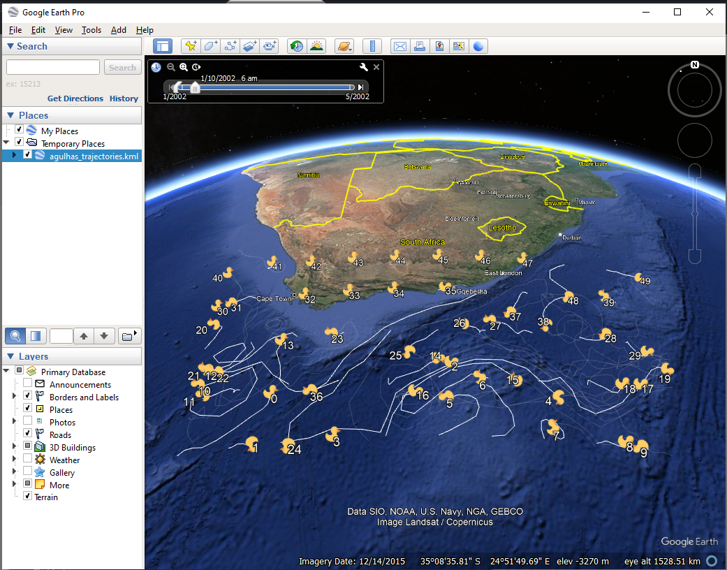
Kepler.gl#
Kepler.gl is a data-agnostic, high-performance web-based application for visual exploration of large-scale geolocation data sets. Built on top of Mapbox GL and deck.gl, kepler.gl can render millions of points representing thousands of trips and perform spatial aggregations on the fly
For smaller visualizations, using the Kepler demo web interface is enough. To animate trips/trajectories in the web interface some customisation to the geojson file is required.
In order to animate the path, the geoJSON data needs to contain
LineStringin its feature geometry, and the coordinates in the LineString need to have 4 elements in the formats of[longitude, latitude, altitude, timestamp]with the last element being a timestamp. Valid timestamp formats include unix in seconds such as1564184363or in milliseconds such as1564184363000.
Kepler.gl tooltip
To do this, we can’t use the same approach as before (as LineString from shapely takes a maximum of 3 values). We instead create the geojson manually.
[9]:
def create_feature_geojson(properties, coordinates):
    """Helper function for creating Kepler geojson"""
    return {
        "type": "Feature",
        "properties": {**properties},
        "geometry": {"type": "LineString", "coordinates": coordinates},
    }


def create_kepler_geojson(gdf, path):
    """
    Converts the GeoDataFrame from the `parcels_to_geopandas` function into geojson
    compatible with the Kepler online viewer, and writes it to a path.

    Parameters
    ----------
    gdf : gpd.GeoDataFrame
        GeoDataFrame as output from the `parcels_to_geopandas` function

    path : pathlike
        Path to save the Kepler geojson to.
    """
    features = []
    for trajectory_idx, trajectory_gdf in gdf.groupby("trajectory"):
        trajectory_gdf = trajectory_gdf.sort_values("obs")

        # Extracting point coordinates
        trajectory_gdf["epoch"] = (
            trajectory_gdf["time"] - datetime.datetime(1970, 1, 1)
        ).dt.total_seconds()
        coordinates = [
            [float(row["geometry"].x), float(row["geometry"].y), 0, int(row["epoch"])]
            for _, row in trajectory_gdf.iterrows()
        ]

        feature_geojson = create_feature_geojson(
            {"pid": int(trajectory_gdf.iloc[0]["trajectory"])}, coordinates
        )
        features.append(feature_geojson)

    kepler_geojson = {"type": "FeatureCollection", "features": features}
    with open(path, "w") as f:
        json.dump(kepler_geojson, f)
    return
[10]:
create_kepler_geojson(
    gdf_parcels, DATA_OUTPUT_FOLDER / f"{DATA_OUTPUT_NAME}_kepler.geojson"
)
We can then load this into the Kepler.gl website. The format of the geojson will be recognised as “Path” for the layer. To get good visuals, its important to tweak the display:
Trail length (measured in seconds)
Trail width
Color (can also color by attribute in the data. E.g. color by particle ID)
For this simulation, a trail length of 2 day (172800 seconds) provides good visuals.
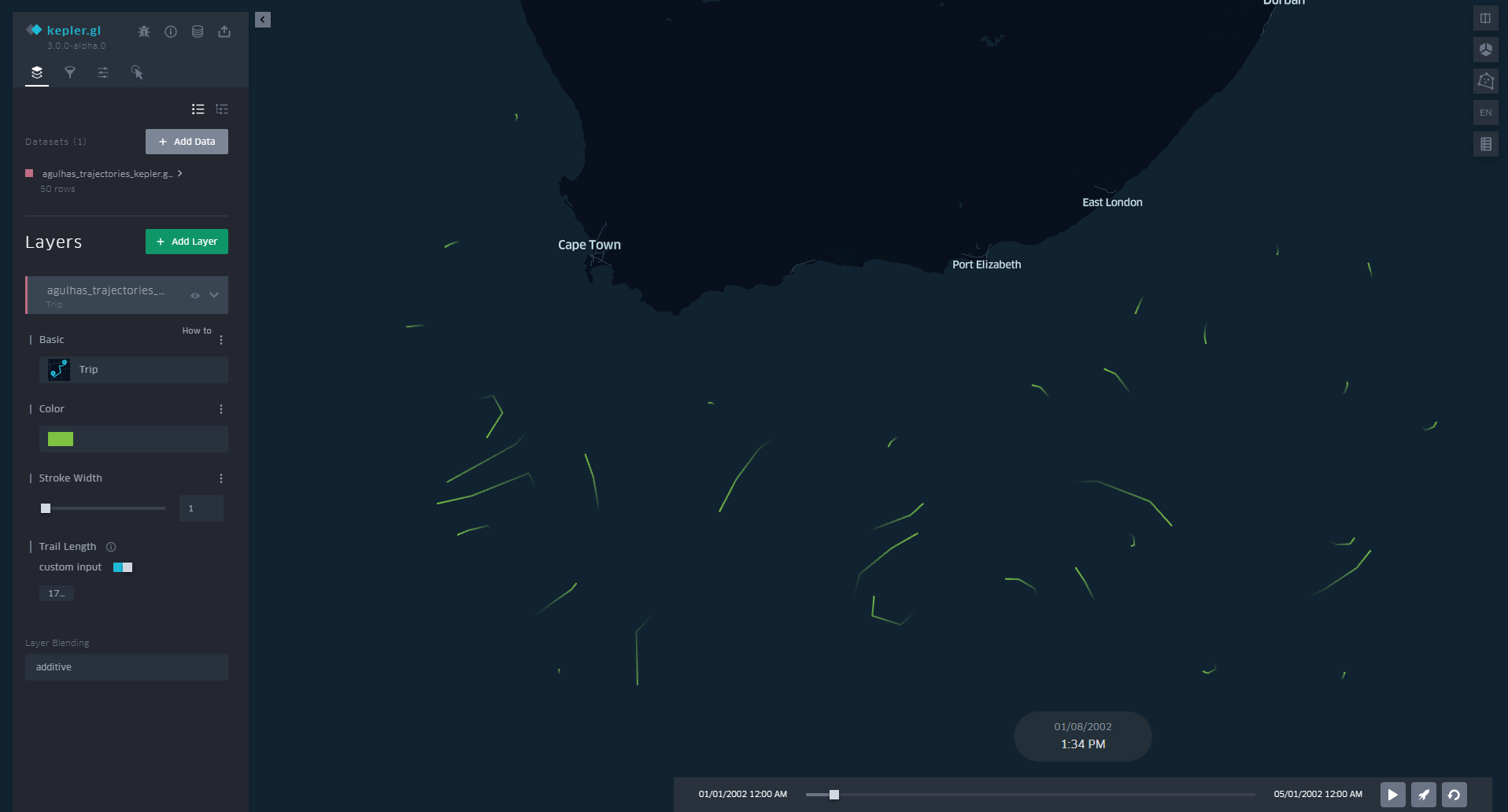
Now we can visualize our trajectories in Kepler!!
Example: Filtering particles by starting location#
Now that we have our parcels data in a geodataframe, we can perform spatial operations with the trajectory output and other datasets. This enables deeper geospatial analysis of particle trajectories, examples including:
Finding particles that start in geographic regions
Finding particles that end in geographic regions
Finding particles that enter within
xkm of a coastline.
In this worked example, we simply want to find out which of the particles start on land so we can exclude them from the analysis.
The steps we follow are:
Step 1: Obtain our geospatial dataset we want to compare against
Here we use ESRI’s World Countries Dataset in geojson format to get polygons of the countries. Alternatively you can create your own polygons in GIS software and export as geojson/shapefile/geopackage for use in Python.
Step 2: Filter observations to get first observation only for each particle
Step 3: Spatial join our data
Step 4: Filter observations to get only the particles in the water
Step 5: Use particle IDs to subset the original xarray dataset, which can be further analyzed.
[11]:
# Step 1: Obtain our geospatial datasets we want to compare against
esri_dataset_url = "https://services.arcgis.com/P3ePLMYs2RVChkJx/arcgis/rest/services/World_Countries_(Generalized)/FeatureServer/0/query?outFields=*&where=1%3D1&f=geojson"

response = requests.get(esri_dataset_url)
if response.status_code == 200:
    geojson_data = response.json()
else:
    raise Exception(
        f"Failed data request for {esri_dataset_url}. Status code {response.status_code}"
    )

gdf_countries = gpd.GeoDataFrame.from_features(geojson_data["features"]).set_crs(
    "EPSG:4326"
)
gdf_countries.head()
[11]:
| geometry | FID | COUNTRY | ISO | COUNTRYAFF | AFF_ISO | Shape__Area | Shape__Length | |
|---|---|---|---|---|---|---|---|---|
| 0 | POLYGON ((61.27655 35.60725, 61.29638 35.62854... | 1 | Afghanistan | AF | Afghanistan | AF | 9.346494e+11 | 6.110457e+06 |
| 1 | POLYGON ((19.57083 41.68527, 19.58195 41.69569... | 2 | Albania | AL | Albania | AL | 5.058670e+10 | 1.271948e+06 |
| 2 | POLYGON ((4.60335 36.88791, 4.63555 36.88638, ... | 3 | Algeria | DZ | Algeria | DZ | 3.014489e+12 | 8.316049e+06 |
| 3 | POLYGON ((-170.74390 -14.37555, -170.74942 -14... | 4 | American Samoa | AS | United States | US | 1.754581e+08 | 6.729120e+04 |
| 4 | POLYGON ((1.44584 42.60194, 1.48653 42.65042, ... | 5 | Andorra | AD | Andorra | AD | 9.349956e+08 | 1.171375e+05 |
[12]:
# Step 2: Filter observations to get first observation only for each particle
gdf_parcels_initial = gdf_parcels.drop_duplicates(subset="trajectory", keep="first")

# Step 3: Spatial join our data
gdf_parcels_initial = gdf_parcels_initial.sjoin(
    gdf_countries[["geometry", "COUNTRY"]], how="left", predicate="intersects"
)
gdf_parcels_initial.tail()
[12]:
| trajectory | obs | time | z | geometry | index_right | COUNTRY | |
|---|---|---|---|---|---|---|---|
| 5445 | 45 | 0 | 2002-01-01 | 0.0 | POINT (25.00000 -32.00000) | 209.0 | South Africa |
| 5566 | 46 | 0 | 2002-01-01 | 0.0 | POINT (27.00000 -32.00000) | 209.0 | South Africa |
| 5687 | 47 | 0 | 2002-01-01 | 0.0 | POINT (29.00000 -32.00000) | 209.0 | South Africa |
| 5808 | 48 | 0 | 2002-01-01 | 0.0 | POINT (31.00000 -32.00000) | NaN | NaN |
| 5929 | 49 | 0 | 2002-01-01 | 0.0 | POINT (33.00000 -32.00000) | NaN | NaN |
[13]:
# Step 4: Filter observations to get only the particles in the water
water_particles_mask = gdf_parcels_initial["COUNTRY"].isna()

particles_in_water = gdf_parcels_initial[water_particles_mask]["trajectory"].values
particles_on_land = gdf_parcels_initial[~water_particles_mask]["trajectory"].values

print(
    f"Particles with the following trajectory IDs are start in water:\n{particles_in_water}\n"
)
print(
    f"Particles with the following trajectory IDs are start on land:\n{particles_on_land}"
)
Particles with the following trajectory IDs are start in water:
[ 0  1  2  3  4  5  6  7  8  9 10 11 12 13 14 15 16 17 18 19 20 21 22 23
 24 25 26 27 28 29 30 31 35 36 37 38 39 40 41 48 49]

Particles with the following trajectory IDs are start on land:
[32 33 34 42 43 44 45 46 47]
These land particles match the particles on land in the Google Earth visualization from earlier.
[14]:
# Step 5: Use particle IDs to subset the original xarray dataset, which can be further analyzed.
ds_parcels_in_water = ds_parcels.sel(trajectory=particles_in_water)

# Continue analysis...
That’s it! You can now integrate Parcels with a variety of geospatial applications.
If there is any additional info, corrections, or geospatial tooling you feel this tutorial can benefit from mentioning, please submit an issue or pull request in the OceanParcels GitHub.