Field Sampling

The particle trajectories allow us to study fields like temperature, plastic concentration or chlorophyll from a Lagrangian perspective.

In this tutorial we will go through how particles can sample Fields, using temperature as an example. Along the way we will get to know the parcels class Variable (see here for the documentation) and some of its methods. This tutorial covers several applications of a sampling setup:

• Basic along trajectory sampling

• Sampling velocity fields

• Sampling initial conditions

• Sampling initial and along-trajectory values with repeated release

Basic sampling

We import the Variable class as well as the standard modules needed to set up a simulation.

# Modules needed for the Parcels simulation
from datetime import timedelta as delta

import matplotlib as mpl
import matplotlib.pyplot as plt
import numpy as np

# To open and look at the temperature data
import xarray as xr

from parcels import (
    AdvectionRK4,
    FieldSet,
    JITParticle,
    ParticleSet,
    Variable,
    download_example_dataset,
)

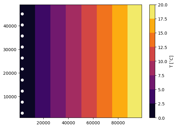
Suppose we want to study the environmental temperature for plankton drifting around a peninsula. We have a dataset with surface ocean velocities and the corresponding sea surface temperature stored in netcdf files in the folder "Peninsula_data". Besides the velocity fields, we load the temperature field using extra_fields={'T': 'T'}. The particles are released on the left hand side of the domain.

# Velocity and temperature fields
example_dataset_folder = download_example_dataset("Peninsula_data")
fieldset = FieldSet.from_parcels(
    f"{example_dataset_folder}/peninsula",
    extra_fields={"T": "T"},
    allow_time_extrapolation=True,
)

# Particle locations and initial time
npart = 10  # number of particles to be released
lon = 3e3 * np.ones(npart)
lat = np.linspace(3e3, 45e3, npart, dtype=np.float32)
time = (
    np.arange(0, npart) * delta(hours=2).total_seconds()
)  # release each particle two hours later

# Plot temperature field and initial particle locations
T_data = xr.open_dataset(f"{example_dataset_folder}/peninsulaT.nc")
plt.figure()
ax = plt.axes()
T_contour = ax.contourf(
    T_data.x.values, T_data.y.values, T_data.T.values[0, 0], cmap=plt.cm.inferno
)
ax.scatter(lon, lat, c="w")
plt.colorbar(T_contour, label="T [$^{\circ} C$]")
plt.show()

To sample the temperature field, we need to create a new class of particles where temperature is a Variable. As an argument for the Variable class, we need to provide the initial values for the particles. The easiest option is to access fieldset.T, but this option has some drawbacks.

class SampleParticle(JITParticle):  # Define a new particle class
    temperature = Variable(
        "temperature", initial=fieldset.T
    )  # Variable 'temperature' initialised by sampling the temperature


pset = ParticleSet(
    fieldset=fieldset, pclass=SampleParticle, lon=lon, lat=lat, time=time
)

WARNING: Particle initialisation from field can be very slow as it is computed in scipy mode.

Using fieldset.T leads to the WARNING displayed above because Variable accesses the fieldset in the slower SciPy mode. Another problem can occur when using the repeatdt argument instead of time:

repeatdt = delta(hours=3)

pset = ParticleSet(
    fieldset=fieldset, pclass=SampleParticle, lon=lon, lat=lat, repeatdt=repeatdt
)

---------------------------------------------------------------------------
RuntimeError                              Traceback (most recent call last)
/Users/erik/Codes/ParcelsCode/docs/examples/tutorial_sampling.ipynb Cell 10 in <cell line: 3>()
      <a href='vscode-notebook-cell:/Users/erik/Codes/ParcelsCode/docs/examples/tutorial_sampling.ipynb#X12sZmlsZQ%3D%3D?line=0'>1</a> repeatdt = delta(hours=3)
----> <a href='vscode-notebook-cell:/Users/erik/Codes/ParcelsCode/docs/examples/tutorial_sampling.ipynb#X12sZmlsZQ%3D%3D?line=2'>3</a> pset = ParticleSet(
      <a href='vscode-notebook-cell:/Users/erik/Codes/ParcelsCode/docs/examples/tutorial_sampling.ipynb#X12sZmlsZQ%3D%3D?line=3'>4</a>     fieldset=fieldset, pclass=SampleParticle, lon=lon, lat=lat, repeatdt=repeatdt
      <a href='vscode-notebook-cell:/Users/erik/Codes/ParcelsCode/docs/examples/tutorial_sampling.ipynb#X12sZmlsZQ%3D%3D?line=4'>5</a> )

File ~/Codes/ParcelsCode/parcels/particleset/particlesetsoa.py:198, in ParticleSetSOA.__init__(self, fieldset, pclass, lon, lat, depth, time, repeatdt, lonlatdepth_dtype, pid_orig, interaction_distance, periodic_domain_zonal, **kwargs)
    190 # The _dirty_neighbor attribute keeps track of whether
    191 # the neighbor search structure needs to be rebuilt.
    192 # If indices change (for example adding/deleting a particle)
    193 # The NS structure needs to be rebuilt and _dirty_neighbor should be
    194 # set to true. Since the NS structure isn't immediately initialized,
    195 # it is set to True here.
    196 self._dirty_neighbor = True
--> 198 self._collection = ParticleCollectionSOA(
    199     _pclass, lon=lon, lat=lat, depth=depth, time=time,
    200     lonlatdepth_dtype=lonlatdepth_dtype, pid_orig=pid_orig,
    201     partitions=partitions, ngrid=ngrids, **kwargs)
    203 # Initialize neighbor search data structure (used for interaction).
    204 if interaction_distance is not None:

File ~/Codes/ParcelsCode/parcels/collection/collectionsoa.py:153, in ParticleCollectionSOA.__init__(self, pclass, lon, lat, depth, time, lonlatdepth_dtype, pid_orig, partitions, ngrid, **kwargs)
    151 for i in range(self.ncount):
    152     if (time[i] is None) or (np.isnan(time[i])):
--> 153         raise RuntimeError(f'Cannot initialise a Variable with a Field if no time provided (time-type: {type(time)} values: {time}). Add a "time=" to ParticleSet construction')
    154     v.initial.fieldset.computeTimeChunk(time[i], 0)
    155     self._data[v.name][i] = v.initial[
    156         time[i], depth[i], lat[i], lon[i]
    157     ]

RuntimeError: Cannot initialise a Variable with a Field if no time provided (time-type: <class 'numpy.ndarray'> values: [None None None None None None None None None None]). Add a "time=" to ParticleSet construction

Since the initial time is not defined, the Variable class does not know at what time to access the temperature field.

The solution to this initialisation problem is to leave the initial value zero and sample the initial condition in JIT mode with the sampling Kernel:

class SampleParticleInitZero(JITParticle):
    """Define a new particle class with Variable 'temperature' init 0"""

    temperature = Variable("temperature", initial=0)


pset = ParticleSet(
    fieldset=fieldset, pclass=SampleParticleInitZero, lon=lon, lat=lat, time=time
)


def SampleT(particle, fieldset, time):
    particle.temperature = fieldset.T[time, particle.depth, particle.lat, particle.lon]


sample_kernel = pset.Kernel(SampleT)  # Casting the SampleT function to a kernel.

To sample the initial values we can execute the Sample kernel over the entire particleset with dt = 0 so that time does not increase

# only execute the sample kernel to record the init temp of the particles
pset.execute(sample_kernel, dt=0)

output_file = pset.ParticleFile(name="InitZero.zarr", outputdt=delta(hours=1))

pset.execute(
    AdvectionRK4 + sample_kernel,
    runtime=delta(hours=30),
    dt=delta(minutes=5),
    output_file=output_file,
)

INFO: Compiled ArraySampleParticleInitZeroSampleT ==> /var/folders/1n/500ln6w97859_nqq86vwpl000000gr/T/parcels-504/lib54c5fd48ca84e26b37f1681b0d1fa1e0_0.so
WARNING: dt or runtime are zero, or endtime is equal to Particle.time. The kernels will be executed once, without incrementing time
INFO: Compiled ArraySampleParticleInitZeroAdvectionRK4SampleT ==> /var/folders/1n/500ln6w97859_nqq86vwpl000000gr/T/parcels-504/lib8300e193dd4e714d46b05efd36dd06b5_0.so

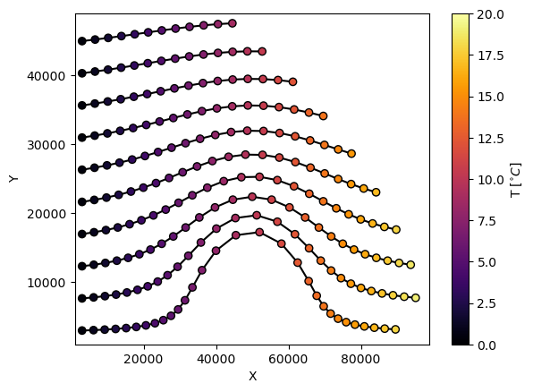
The particle dataset now contains the particle trajectories and the corresponding environmental temperature

Particle_data = xr.open_zarr("InitZero.zarr")

plt.figure()
ax = plt.axes()
ax.set_ylabel("Y")
ax.set_xlabel("X")
ax.set_ylim(1000, 49000)
ax.set_xlim(1000, 99000)
ax.plot(Particle_data.lon.transpose(), Particle_data.lat.transpose(), c="k", zorder=1)
T_scatter = ax.scatter(
    Particle_data.lon,
    Particle_data.lat,
    c=Particle_data.temperature,
    cmap=plt.cm.inferno,
    norm=mpl.colors.Normalize(vmin=0.0, vmax=20.0),
    edgecolor="k",
    zorder=2,
)
plt.colorbar(T_scatter, label="T [$^{\circ} C$]")
plt.show()

Sampling velocity fields

Because Parcels works also for generalised curvilinear grids, you need to tread somewhat carefully when wanting to sample the velocity fields U and V. In fact, Parcels will throw a warning when directly calling a sampling of either of these fields:

def SampleVel_wrong(particle, fieldset, time):
    u = fieldset.U[particle]


pset = ParticleSet(fieldset=fieldset, pclass=JITParticle, lon=lon, lat=lat, time=time)

pset.execute(SampleVel_wrong)

WARNING: Sampling of velocities should normally be done using fieldset.UV or fieldset.UVW object; thread carefully
INFO: Compiled ArrayJITParticleSampleVel_wrong ==> /var/folders/1n/500ln6w97859_nqq86vwpl000000gr/T/parcels-504/libbb7475bee9a1576ca3a79c9b70b5f23e_0.so

Instead, you should use the code u, v = fieldset.UV[...]. With this code, the sampling is consistent with the actual velocity fields used in the advection Kernels. The difference is that on a curvilinear grid, fieldset.U[..] returns the velocity in the i-direction (the columns on the grid), while fieldset.UV[...] returns the velocities in the longitude and latitude direction. Furthermore, only fieldset.UV[...] sampling can correctly deal with boundary conditions such as freeslip and partialslip (documentation_unstuck_Agrid)

def SampleVel_correct(particle, fieldset, time):
    u, v = fieldset.UV[particle]


pset = ParticleSet(fieldset=fieldset, pclass=JITParticle, lon=lon, lat=lat, time=time)

pset.execute(SampleVel_correct)

INFO: Compiled ArrayJITParticleSampleVel_correct ==> /var/folders/1n/500ln6w97859_nqq86vwpl000000gr/T/parcels-504/lib8eff8d1a0b188ff800a066f2e9ab4ef8_0.so

To sample U and V as part of a larger script the following code could be used:

class SampleParticle(JITParticle):
    U = Variable("U", dtype=np.float32, initial=np.nan)
    V = Variable("V", dtype=np.float32, initial=np.nan)


def SampleVel_correct(particle, fieldset, time):
    # attention: samples particle velocity in units of the mesh (deg/s or m/s)
    particle.U, particle.V = fieldset.UV[
        time, particle.depth, particle.lat, particle.lon, particle
    ]

Sampling initial values

In some simulations only the particles initial value within the field is of interest: the variable does not need to be known along the entire trajectory. To reduce computing we can specify the to_write argument to the temperature Variable. This argument can have three values: True, False or 'once'. It determines whether to write the Variable to the output file. If we want to know only the initial value, we can enter 'once' and only the first value will be written to the output file.

class SampleParticleOnce(JITParticle):
    """Define a new particle class with Variable 'temperature'
    initially zero and only written once"""

    temperature = Variable("temperature", initial=0, to_write="once")


pset = ParticleSet(
    fieldset=fieldset, pclass=SampleParticleOnce, lon=lon, lat=lat, time=time
)

# only execute the sample kernel to record the init temp of the particles
pset.execute(sample_kernel, dt=0)

output_file = pset.ParticleFile(name="WriteOnce.zarr", outputdt=delta(hours=1))

pset.execute(
    AdvectionRK4, runtime=delta(hours=24), dt=delta(minutes=5), output_file=output_file
)

INFO: Compiled ArraySampleParticleInitZeroSampleT ==> /var/folders/1n/500ln6w97859_nqq86vwpl000000gr/T/parcels-504/lib7068bde278d3b088dcf0c9c51ceb4980_0.so
INFO: Compiled ArraySampleParticleOnceAdvectionRK4 ==> /var/folders/1n/500ln6w97859_nqq86vwpl000000gr/T/parcels-504/lib590e70b310a52a3d0e0a583012301d4d_0.so

Since all the particles are released at the same x-position and the temperature field is invariant in the y-direction, all particles have an initial temperature of 0.4\(^\circ\)C

Particle_data = xr.open_zarr("WriteOnce.zarr")

plt.figure()
ax = plt.axes()
ax.set_ylabel("Y")
ax.set_xlabel("X")
ax.set_ylim(1000, 49000)
ax.set_xlim(1000, 99000)
ax.plot(Particle_data.lon.transpose(), Particle_data.lat.transpose(), c="k", zorder=1)
T_scatter = ax.scatter(
    Particle_data.lon,
    Particle_data.lat,
    c=np.tile(Particle_data.temperature, (Particle_data.lon.shape[1], 1)).T,
    cmap=plt.cm.inferno,
    norm=mpl.colors.Normalize(vmin=0.0, vmax=1.0),
    edgecolor="k",
    zorder=2,
)
plt.colorbar(T_scatter, label="Initial T [$^{\circ} C$]")
plt.show()

Sampling with repeatdt

Some experiments require large sets of particles to be released repeatedly on the same locations. The particleset object has the option repeatdt for this, but when you want to sample the initial values this introduces some problems as we have seen above in the error when using repeatdt. For more advanced control over the repeated release of particles, you can manually write a for-loop using the function particleset.add(). Note that this for-loop is very similar to the one that repeatdt would execute under the hood in particleset.execute().

Adding particles to the particleset during the simulation reduces the memory used compared to specifying the delayed particle release times upfront, which improves the computational speed. In the loop, we want to initialise new particles and sample their initial temperature. If we want to write both the initialised particles with the sampled temperature and the older particles that have already been advected, we have to make sure both sets of particles find themselves at the same moment in time. The initial conditions must be written to the output file before advecting them, because during advection the particle.time will increase.

We do not specify the outputdt argument for the output_file and instead write the data with output_file.write(pset, time) on each iteration. A new particleset is initialised whenever time is a multiple of repeatdt. Because the particles are advected after being written, the last displacement must be written once more after the loop.

# write the particle data every hour
outputdt = delta(hours=1).total_seconds()

# release each set of particles six hours later
repeatdt = delta(hours=6).total_seconds()

# run the model for 24 hours
runtime = delta(hours=24).total_seconds()

pset = ParticleSet(
    fieldset=fieldset, pclass=SampleParticleInitZero, lon=[], lat=[], time=[]
)
kernels = AdvectionRK4 + sample_kernel

# Note: Do not specify the outputdt yet, so we can manually write the output
output_file = pset.ParticleFile(name="RepeatLoop.zarr")

for time in np.arange(0, runtime, outputdt):
    # check if time is a multiple of repeatdt
    if np.isclose(np.fmod(time, repeatdt), 0):
        pset_init = ParticleSet(
            fieldset=fieldset,
            pclass=SampleParticleInitZero,
            lon=lon,
            lat=lat,
            time=time,
        )
        # record the initial temperature of the particles
        pset_init.execute(sample_kernel, dt=0)

        # add the newly released particles to the total particleset
        pset.add(pset_init)

    # write the initialised particles and the advected particles
    output_file.write(pset, time)

    pset.execute(kernels, runtime=outputdt, dt=delta(minutes=5))
    print(f"Length of pset at time {time}: {len(pset)}")

output_file.write(pset, time + outputdt)

INFO: Compiled ArraySampleParticleInitZeroSampleT ==> /var/folders/1n/500ln6w97859_nqq86vwpl000000gr/T/parcels-504/lib9d9b0cd4049228e1cfe32eeb52d883e5_0.so
INFO: Compiled ArraySampleParticleInitZeroAdvectionRK4SampleT ==> /var/folders/1n/500ln6w97859_nqq86vwpl000000gr/T/parcels-504/lib439c24428fc59a3002424fbbe2260805_0.so
Length of pset at time 0.0: 10
Length of pset at time 3600.0: 10
Length of pset at time 7200.0: 10
Length of pset at time 10800.0: 10
Length of pset at time 14400.0: 10
Length of pset at time 18000.0: 10
INFO: Compiled ArraySampleParticleInitZeroSampleT ==> /var/folders/1n/500ln6w97859_nqq86vwpl000000gr/T/parcels-504/lib68bdb1261df815a56477b7357a120618_0.so
Length of pset at time 21600.0: 20
Length of pset at time 25200.0: 20
Length of pset at time 28800.0: 20
Length of pset at time 32400.0: 20
Length of pset at time 36000.0: 20
Length of pset at time 39600.0: 20
INFO: Compiled ArraySampleParticleInitZeroSampleT ==> /var/folders/1n/500ln6w97859_nqq86vwpl000000gr/T/parcels-504/lib8ea2664f9d6e608afa3bfa2513b7b39f_0.so
Length of pset at time 43200.0: 30
Length of pset at time 46800.0: 30
Length of pset at time 50400.0: 30
Length of pset at time 54000.0: 30
Length of pset at time 57600.0: 30
Length of pset at time 61200.0: 30
INFO: Compiled ArraySampleParticleInitZeroSampleT ==> /var/folders/1n/500ln6w97859_nqq86vwpl000000gr/T/parcels-504/libb1032682b9b16901cecda62ec609f5c3_0.so
Length of pset at time 64800.0: 40
Length of pset at time 68400.0: 40
Length of pset at time 72000.0: 40
Length of pset at time 75600.0: 40
Length of pset at time 79200.0: 40
Length of pset at time 82800.0: 40

In each iteration of the loop, spanning six hours, we have added ten particles.

Particle_data = xr.open_zarr("RepeatLoop.zarr")
print(
    Particle_data.time[:, 0].values / np.timedelta64(1, "h")
)  # The initial hour at which each particle is released
assert np.allclose(
    Particle_data.time[:, 0].values / np.timedelta64(1, "h"),
    [int(k / 10) * 6 for k in range(40)],
)

[ 0.  0.  0.  0.  0.  0.  0.  0.  0.  0.  6.  6.  6.  6.  6.  6.  6.  6.
  6.  6. 12. 12. 12. 12. 12. 12. 12. 12. 12. 12. 18. 18. 18. 18. 18. 18.
 18. 18. 18. 18.]

Let’s check if the initial temperatures were sampled correctly for all particles

print(Particle_data.temperature[:, 0].values)
assert np.allclose(
    Particle_data.temperature[:, 0].values, Particle_data.temperature[:, 0].values[0]
)

[0.4040816 0.4040816 0.4040816 0.4040816 0.4040816 0.4040816 0.4040816
 0.4040816 0.4040816 0.4040816 0.4040816 0.4040816 0.4040816 0.4040816
 0.4040816 0.4040816 0.4040816 0.4040816 0.4040816 0.4040816 0.4040816
 0.4040816 0.4040816 0.4040816 0.4040816 0.4040816 0.4040816 0.4040816
 0.4040816 0.4040816 0.4040816 0.4040816 0.4040816 0.4040816 0.4040816
 0.4040816 0.4040816 0.4040816 0.4040816 0.4040816]

And see if the sampling of the temperature field is done correctly along the trajectories

Release0 = Particle_data.where(
    Particle_data.time[:, 0] == np.timedelta64(0, "s")
)  # the particles released at t = 0

plt.figure()
ax = plt.axes()
ax.set_ylabel("Y")
ax.set_xlabel("X")
ax.set_ylim(1000, 49000)
ax.set_xlim(1000, 99000)
ax.plot(Release0.lon.transpose(), Release0.lat.transpose(), c="k", zorder=1)
T_scatter = ax.scatter(
    Release0.lon,
    Release0.lat,
    c=Release0.temperature,
    cmap=plt.cm.inferno,
    norm=mpl.colors.Normalize(vmin=0.0, vmax=20.0),
    edgecolor="k",
    zorder=2,
)
plt.colorbar(T_scatter, label="T [$^{\circ} C$]")
plt.show()