Working with Parcels output

This tutorial covers the format of the trajectory output exported by Parcels. Parcels does not include advanced analysis or plotting functionality, which users are suggested to write themselves to suit their research goals. Here we provide some starting points to explore the parcels output files yourself.

• Reading the output file

• Trajectory data structure

• Analysis

• Plotting

• Animations

First we need to create some parcels output to analyze. We simulate a set of particles using the setup described in the Delay start tutorial.

from datetime import timedelta as delta

import numpy as np

from parcels import (
    AdvectionRK4,
    FieldSet,
    JITParticle,
    ParticleSet,
    download_example_dataset,
)

example_dataset_folder = download_example_dataset("Peninsula_data")
fieldset = FieldSet.from_parcels(
    f"{example_dataset_folder}/peninsula", allow_time_extrapolation=True
)

npart = 10  # number of particles to be released
lon = 3e3 * np.ones(npart)
lat = np.linspace(3e3, 45e3, npart, dtype=np.float32)

# release every particle two hours later
time = np.arange(npart) * delta(hours=2).total_seconds()

pset = ParticleSet(fieldset=fieldset, pclass=JITParticle, lon=lon, lat=lat, time=time)

output_file = pset.ParticleFile(name="Output.zarr", outputdt=delta(hours=2))

pset.execute(
    AdvectionRK4, runtime=delta(hours=24), dt=delta(minutes=5), output_file=output_file
)

INFO: Output files are stored in Output.zarr.
100%|██████████| 86400.0/86400.0 [00:00<00:00, 93792.23it/s]

Reading the output file

Parcels exports output trajectories in zarr format. Files in zarr are typically much smaller in size than netcdf, although may be slightly more challenging to handle (but xarray has a fairly seamless open_zarr() method).

import xarray as xr

data_xarray = xr.open_zarr("Output.zarr")
print(data_xarray)

<xarray.Dataset>
Dimensions:     (trajectory: 10, obs: 12)
Coordinates:
  * obs         (obs) int32 0 1 2 3 4 5 6 7 8 9 10 11
  * trajectory  (trajectory) int64 0 1 2 3 4 5 6 7 8 9
Data variables:
    lat         (trajectory, obs) float32 dask.array<chunksize=(1, 1), meta=np.ndarray>
    lon         (trajectory, obs) float32 dask.array<chunksize=(1, 1), meta=np.ndarray>
    time        (trajectory, obs) timedelta64[ns] dask.array<chunksize=(1, 1), meta=np.ndarray>
    z           (trajectory, obs) float32 dask.array<chunksize=(1, 1), meta=np.ndarray>
Attributes:
    Conventions:            CF-1.6/CF-1.7
    feature_type:           trajectory
    ncei_template_version:  NCEI_NetCDF_Trajectory_Template_v2.0
    parcels_kernels:        JITParticleAdvectionRK4
    parcels_mesh:           flat
    parcels_version:        v2.4.2-367-gd9b7b447

print(data_xarray["trajectory"])

<xarray.DataArray 'trajectory' (trajectory: 10)>
array([0, 1, 2, 3, 4, 5, 6, 7, 8, 9])
Coordinates:
  * trajectory  (trajectory) int64 0 1 2 3 4 5 6 7 8 9

Note that if you are running Parcels on multiple processors with mpirun, you will need to concatenate the files of each processor, see also the MPI documentation.

Also, once you have loaded the data as an xarray DataSet using xr.open_zarr(), you can always save the file to NetCDF if you prefer with the .to_netcdf() method.

Trajectory data structure

The data zarr file are organised according to the CF-conventions implemented with the NCEI trajectory template. The data is stored in a two-dimensional array with the dimensions traj and obs. Each particle trajectory is essentially stored as a time series where the coordinate data (lon, lat, time) are a function of the observation (obs).

The output dataset used here contains 10 particles and 13 observations. Not every particle has 13 observations however; since we released particles at different times some particle trajectories are shorter than others.

np.set_printoptions(linewidth=160)
ns_per_hour = np.timedelta64(1, "h")  # nanoseconds in an hour

print(data_xarray["time"].data.compute() / ns_per_hour)  # time is stored in nanoseconds

[[ 0.  2.  4.  6.  8. 10. 12. 14. 16. 18. 20. 22.]
 [ 2.  4.  6.  8. 10. 12. 14. 16. 18. 20. 22. nan]
 [ 4.  6.  8. 10. 12. 14. 16. 18. 20. 22. nan nan]
 [ 6.  8. 10. 12. 14. 16. 18. 20. 22. nan nan nan]
 [ 8. 10. 12. 14. 16. 18. 20. 22. nan nan nan nan]
 [10. 12. 14. 16. 18. 20. 22. nan nan nan nan nan]
 [12. 14. 16. 18. 20. 22. nan nan nan nan nan nan]
 [14. 16. 18. 20. 22. nan nan nan nan nan nan nan]
 [16. 18. 20. 22. nan nan nan nan nan nan nan nan]
 [18. 20. 22. nan nan nan nan nan nan nan nan nan]]

Note how the first observation occurs at a different time for each trajectory. So remember that obs != time

Analysis

Sometimes, trajectories are analyzed as they are stored: as individual time series. If we want to study the distance travelled as a function of time, the time we are interested in is the time relative to the start of the each particular trajectory: the array operations are simple since each trajectory is analyzed as a function of obs. The time variable is only needed to express the results in the correct units.

import matplotlib.pyplot as plt

x = data_xarray["lon"].values
y = data_xarray["lat"].values
distance = np.cumsum(
    np.sqrt(np.square(np.diff(x)) + np.square(np.diff(y))), axis=1
)  # d = (dx^2 + dy^2)^(1/2)

real_time = data_xarray["time"] / ns_per_hour  # convert time to hours
time_since_release = (
    real_time.values.transpose() - real_time.values[:, 0]
)  # substract the initial time from each timeseries

fig, (ax1, ax2) = plt.subplots(1, 2, figsize=(10, 4), constrained_layout=True)

ax1.set_ylabel("Distance travelled [m]")
ax1.set_xlabel("observation", weight="bold")
d_plot = ax1.plot(distance.transpose())

ax2.set_ylabel("Distance travelled [m]")
ax2.set_xlabel("time since release [hours]", weight="bold")
d_plot_t = ax2.plot(time_since_release[1:], distance.transpose())
plt.show()

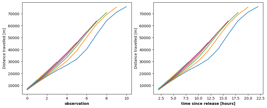
The two figures above show the same graph. Time is not needed to create the first figure. The time variable minus the first value of each trajectory gives the x-axis the correct units in the second figure.

We can also plot the distance travelled as a function of the absolute time easily, since the time variable matches up with the data for each individual trajectory.

plt.figure()
ax = plt.axes()
ax.set_ylabel("Distance travelled [m]")
ax.set_xlabel("time [hours]", weight="bold")
d_plot_t = ax.plot(real_time.T[1:], distance.transpose())

Conditional selection

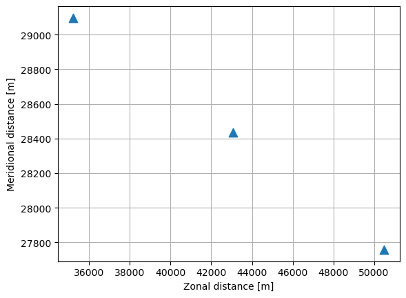
In other cases, the processing of the data itself however depends on the absolute time at which the observations are made, e.g. studying seasonal phenomena. In that case the array structure is not as simple: the data must be selected by their time value. Here we show how the mean location of the particles evolves through time. This also requires the trajectory data to be aligned in time. The data are selected using xr.DataArray.where() which compares the time variable to a specific time. This type of selecting data with a condition (data_xarray['time']==time) is a powerful tool to analyze trajectory data.

# Using xarray
mean_lon_x = []
mean_lat_x = []

timerange = np.arange(
    np.nanmin(data_xarray["time"].values),
    np.nanmax(data_xarray["time"].values) + np.timedelta64(delta(hours=2)),
    delta(hours=2),
)  # timerange in nanoseconds

for time in timerange:
    # if all trajectories share an observation at time
    if np.all(np.any(data_xarray["time"] == time, axis=1)):
        # find the data that share the time
        mean_lon_x += [
            np.nanmean(data_xarray["lon"].where(data_xarray["time"] == time).values)
        ]
        mean_lat_x += [
            np.nanmean(data_xarray["lat"].where(data_xarray["time"] == time).values)
        ]

/Users/erik/miniconda3/envs/parcels/lib/python3.11/site-packages/pandas/core/arrays/timedeltas.py:1093: RuntimeWarning: invalid value encountered in cast
  data = (base * m + (frac * m).astype(np.int64)).view("timedelta64[ns]")

plt.figure()
ax = plt.axes()
ax.set_ylabel("Meridional distance [m]")
ax.set_xlabel("Zonal distance [m]")
ax.grid()
ax.scatter(mean_lon_x, mean_lat_x, marker="^", s=80)
plt.show()

Plotting

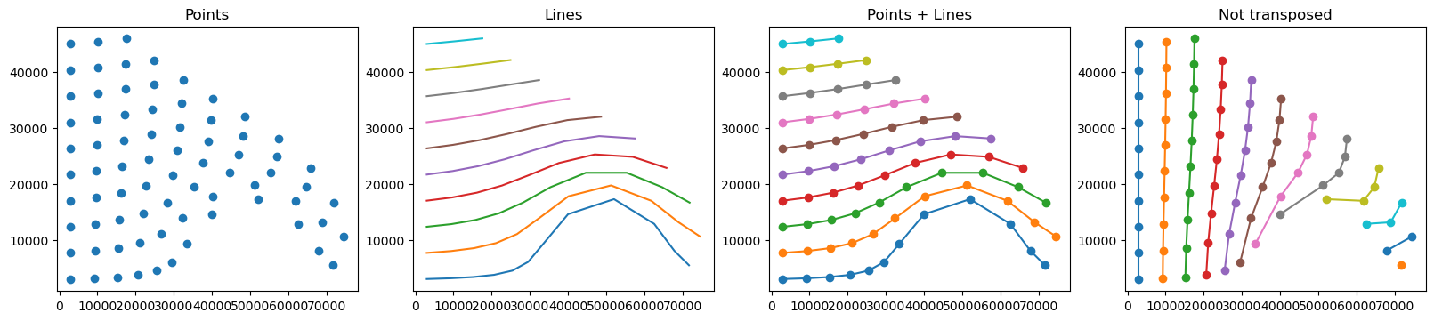
Parcels output consists of particle trajectories through time and space. An important way to explore patterns in this information is to draw the trajectories in space. The trajan package can be used to quickly plot parcels results, but users are encouraged to create their own figures, for example by using the comprehensive matplotlib library. Here we show a basic setup on how to process the parcels output into trajectory plots and animations.

Some other packages to help you make beautiful figures are:

• cartopy, a map-drawing tool especially compatible with matplotlib

• trajan, a package to quickly plot trajectories

• cmocean, a set of ocean-relevant colormaps

To draw the trajectory data in space usually it is informative to draw points at the observed coordinates to see the resolution of the output and draw a line through them to separate the different trajectories. The coordinates to draw are in lon and lat and can be passed to either matplotlib.pyplot.plot or matplotlib.pyplot.scatter. Note however, that the default way matplotlib plots 2D arrays is to plot a separate set for each column. In the parcels 2D output, the columns correspond to the obs dimension, so to separate the different trajectories we need to transpose the 2D array using .T.

fig, (ax1, ax2, ax3, ax4) = plt.subplots(
    1, 4, figsize=(16, 3.5), constrained_layout=True
)

###-Points-###
ax1.set_title("Points")
ax1.scatter(data_xarray["lon"].T, data_xarray["lat"].T)
###-Lines-###
ax2.set_title("Lines")
ax2.plot(data_xarray["lon"].T, data_xarray["lat"].T)
###-Points + Lines-###
ax3.set_title("Points + Lines")
ax3.plot(data_xarray["lon"].T, data_xarray["lat"].T, marker="o")
###-Not Transposed-###
ax4.set_title("Not transposed")
ax4.plot(data_xarray["lon"], data_xarray["lat"], marker="o")

plt.show()

Animations

Trajectory plots like the ones above can become very cluttered for large sets of particles. To better see patterns, it’s a good idea to create an animation in time and space. To do this, matplotlib offers an animation package. Here we show how to use the FuncAnimation class to animate parcels trajectory data.

To correctly reveal the patterns in time we must remember that the obs dimension does not necessarily correspond to the time variable (see the section of Trajectory data structure above). In the animation of the particles, we usually want to draw the points at each consecutive moment in time, not necessarily at each moment since the start of the trajectory. To do this we must select the correct data in each rendering.

from IPython.display import HTML
from matplotlib.animation import FuncAnimation

outputdt = delta(hours=2)

# timerange in nanoseconds
timerange = np.arange(
    np.nanmin(data_xarray["time"].values),
    np.nanmax(data_xarray["time"].values) + np.timedelta64(outputdt),
    outputdt,
)

%%capture
fig = plt.figure(figsize=(5, 5), constrained_layout=True)
ax = fig.add_subplot()

ax.set_ylabel("Meridional distance [m]")
ax.set_xlabel("Zonal distance [m]")
ax.set_xlim(0, 90000)
ax.set_ylim(0, 50000)
plt.xticks(rotation=45)

# Indices of the data where time = 0
time_id = np.where(data_xarray["time"] == timerange[0])

scatter = ax.scatter(
    data_xarray["lon"].values[time_id], data_xarray["lat"].values[time_id]
)

t = str(timerange[0].astype("timedelta64[h]"))
title = ax.set_title("Particles at t = " + t)


def animate(i):
    t = str(timerange[i].astype("timedelta64[h]"))
    title.set_text("Particles at t = " + t)

    time_id = np.where(data_xarray["time"] == timerange[i])
    scatter.set_offsets(
        np.c_[data_xarray["lon"].values[time_id], data_xarray["lat"].values[time_id]]
    )


anim = FuncAnimation(fig, animate, frames=len(timerange), interval=100)

HTML(anim.to_jshtml())

Once Loop Reflect