Parallelisation with MPI and Field chunking with dask

Parcels can be run in Parallel with MPI. To do this, you will need to also install the mpich and mpi4py packages (e.g. conda install mpich mpi4py).

Note that these packages don’t work on Windows, and that they have been installed if you followed the Installation for Developers instructions.

Splitting the ParticleSet with MPI

Once you have installed a parallel version of Parcels, you can simply run your script with

mpirun -np <np> python <yourscript.py>

Where <np> is the number of processors you want to use

Parcels will then split the ParticleSet into <np> smaller ParticleSets, based on a sklearn.cluster.KMeans clustering. Each of those smaller ParticleSets will be executed by one of the <np> MPI processors.

Note that in principle this means that all MPI processors need access to the full FieldSet, which can be Gigabytes in size for large global datasets. Therefore, efficient parallelisation only works if at the same time we also chunk the FieldSet into smaller domains.

Optimising the partitioning of the particles with a user-defined partition_function

Parcels uses so-called partition functions to assign particles to processors. By default, Parcels uses a scikit-learn KMeans clustering algorithm to partition the particles. However, you can also define your own partition function, which can be useful if you know more about the distribution of particles in your domain than the KMeans algorithm does.

To define your own partition function, you need to define a function that takes a list of coordinates (lat, lon) as input, and returns a list of integers, defining the MPI processor that each particle should be assigned to. See the example below:

def simple_partition_function(coords, mpi_size=1):
    """A very simple partition function
    that assigns particles to processors
    """
    return np.linspace(0, mpi_size, coords.shape[0], endpoint=False, dtype=np.int32)

To add the partition function to your script, you need to add it to the ParticleSet constructor:

pset = ParticleSet(..., partition_function=simple_partition_function)

Reading in the ParticleFile data in zarr format

For efficiency, each processor will write its own data to a zarr-store. If the name of your ParticleFile is fname, then these stores will be located at fname/proc00.zarr, fname/proc01.zarr, etc.

Reading in these stores and merging them into one xarray.Dataset can be done with

from glob import glob
from os import path

files = glob(path.join(fname, "proc*"))
ds = xr.concat(
    [xr.open_zarr(f) for f in files],
    dim="trajectory",
    compat="no_conflicts",
    coords="minimal",
)

Note that, if you have added particles during the execute() (for example because you used repeatdt), then the trajectories will not be ordered monotonically. While this may not be a problem, this will result in a different Dataset than a single-core simulation. If you do want the outputs of the MPI run to be the same as the single-core run, add .sortby(['trajectory']) at the end of the xr.concat() command

ds = xr.concat(
    [xr.open_zarr(f) for f in files],
    dim="trajectory",
    compat="no_conflicts",
    coords="minimal",
).sortby(["trajectory"])

Note that if you want, you can save this new DataSet with the .to_zarr() or .to_netcdf() methods.

When using .to_zarr(), then further analysis may be sped up by first rechunking the DataSet, by using ds.chunk(). Note that in some cases, you will first need to remove the chunks encoding information manually, using a code like below

For small projects, the above instructions are sufficient. If your project is large, then it is helpful to combine the proc* directories into a single zarr dataset and to optimise the chunking for your analysis. What is “large”? If you find yourself running out of memory while doing your analysis, saving the results, or sorting the dataset, or if reading the data is taking longer than you can tolerate, your problem is “large.” Another rule of thumb is if the size of your output directory is 1/3 or more of the memory of your machine, your problem is large. Chunking and combining the proc* data in order to speed up analysis is discussed in the documentation on runs with large output.

Chunking the FieldSet with dask

The basic idea of field-chunking in Parcels is that we use the dask library to load only these regions of the Field that are occupied by Particles. The advantage is that if different MPI processors take care of Particles in different parts of the domain, each only needs to load a small section of the full FieldSet (although note that this load-balancing functionality is still in development). Furthermore, the field-chunking in principle makes the indices keyword superfluous, as Parcels will determine which part of the domain to load itself.

The default behaviour is for dask to control the chunking, via a call to da.from_array(data, chunks='auto'). The chunksizes are then determined by the layout of the NetCDF files.

However, in tests we have experienced that this may not necessarily be the most efficient chunking. Therefore, Parcels provides control over the chunksize via the chunksize keyword in Field creation, which requires a dictionary that sets the typical size of chunks for each dimension.

It is strongly encouraged to explore what the best value for chunksize is for your experiment, which will depend on the FieldSet, the ParticleSet and the type of simulation (2D versus 3D). As a guidance, we have found that chunksizes in the zonal and meridional direction of approximately around 128 to 512 are typically most effective. The binning relates to the size of the model and its data size, so power-of-two values are advantageous but not required.

The notebook below shows an example script to explore the scaling of the time taken for pset.execute() as a function of zonal and meridional chunksize for a dataset from the CMEMS portal.

%pylab inline
import os
import time
from datetime import timedelta as delta
from glob import glob

import matplotlib.pyplot as plt
import numpy as np
import psutil

from parcels import AdvectionRK4, FieldSet, JITParticle, ParticleSet


def set_cmems_fieldset(cs):
    data_dir_head = "/data/oceanparcels/input_data"
    data_dir = os.path.join(data_dir_head, "CMEMS/GLOBAL_REANALYSIS_PHY_001_030/")
    files = sorted(glob(data_dir + "mercatorglorys12v1_gl12_mean_201607*.nc"))
    variables = {"U": "uo", "V": "vo"}
    dimensions = {"lon": "longitude", "lat": "latitude", "time": "time"}

    if cs not in ["auto", False]:
        cs = {"time": ("time", 1), "lat": ("latitude", cs), "lon": ("longitude", cs)}
    return FieldSet.from_netcdf(files, variables, dimensions, chunksize=cs)


func_time = []
mem_used_GB = []
chunksize = [128, 256, 512, 768, 1024, 1280, 1536, 1792, 2048, 2610, "auto", False]
for cs in chunksize:
    fieldset = set_cmems_fieldset(cs)
    pset = ParticleSet(
        fieldset=fieldset, pclass=JITParticle, lon=[0], lat=[0], repeatdt=delta(hours=1)
    )

    tic = time.time()
    pset.execute(AdvectionRK4, dt=delta(hours=1))
    func_time.append(time.time() - tic)
    process = psutil.Process(os.getpid())
    mem_B_used = process.memory_info().rss
    mem_used_GB.append(mem_B_used / (1024 * 1024))

Populating the interactive namespace from numpy and matplotlib

fig, ax = plt.subplots(1, 1, figsize=(15, 7))

ax.plot(chunksize[:-2], func_time[:-2], "o-")
ax.plot([0, 2800], [func_time[-2], func_time[-2]], "--", label=chunksize[-2])
ax.plot([0, 2800], [func_time[-1], func_time[-1]], "--", label=chunksize[-1])
plt.xlim([0, 2800])
plt.legend()
ax.set_xlabel("chunksize")
ax.set_ylabel("Time spent in pset.execute() [s]")
plt.show()

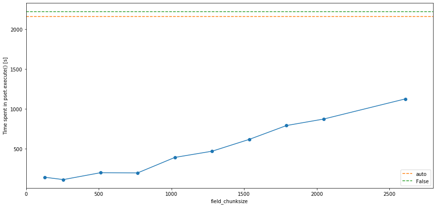
The plot above shows that in this case, chunksize='auto' and chunksize=False (the two dashed lines) are roughly the same speed, but that the fastest run is for chunksize=(1, 256, 256). But note that the actual thresholds and numbers depend on the FieldSet used and the specifics of your experiment.

Furthermore, one of the major advantages of field chunking is the efficient utilization of memory. This permits the distribution of the particle advection to many cores, as otherwise the processing unit (e.g. a CPU core; a node in a cluster) would exhaust the memory rapidly. This is shown in the following plot of the memory behaviour.

fig, ax = plt.subplots(1, 1, figsize=(15, 12))
ax.plot(chunksize[:-2], mem_used_GB[:-2], "--", label="memory_blocked [MB]")
ax.plot([0, 2800], [mem_used_GB[-2], mem_used_GB[-2]], "x-", label="auto [MB]")
ax.plot([0, 2800], [mem_used_GB[-1], mem_used_GB[-1]], "--", label="no chunking [MB]")
plt.legend()
ax.set_xlabel("chunksize")
ax.set_ylabel("Memory blocked in pset.execute() [MB]")
plt.show()

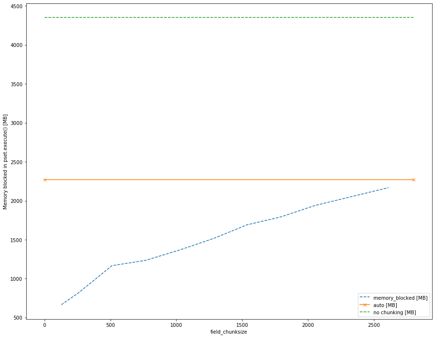
It can clearly be seen that with chunksize=False (green line), all Field data are loaded in full directly into memory, which can lead to MPI-run simulations being aborted for memory reasons. Furthermore, one can see that even the automatic method is not optimal, and optimizing the chunksize for a specific hydrodynamic dataset can make a large difference to the memory used.

It may - depending on your simulation goal - be necessary to tweak the chunksize to leave more memory space for additional particles that are being simulated. Since particles and fields share the same memory space, lower memory utilisation by the FieldSet means more memory available for a larger ParticleSet.

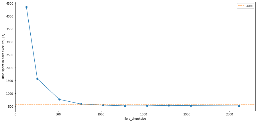
Also note that the above example is for a 2D application. For 3D applications, the chunksize=False will almost always be slower than chunksize='auto' or any dictionary, and is likely to run into insufficient memory issues, raising a MemoryError. The plot below shows the same analysis as above, but this time for a set of simulations using the full 3D CMEMS code. In this case, the chunksize='auto' is about two orders of magnitude faster than running without chunking, and about 7.5 times faster than with minimal chunk capacity (i.e. chunksize=(1, 128, 128)).

Choosing too small chunksizes can make the code slower, again highlighting that it is wise to explore which chunksize is best for your experiment before you perform it.

from parcels import AdvectionRK4_3D


def set_cmems_fieldset_3D(cs):
    data_dir_head = "/data/oceanparcels/input_data"
    data_dir = os.path.join(data_dir_head, "CMEMS/GLOBAL_REANALYSIS_PHY_001_030/")
    files = sorted(glob(data_dir + "mercatorglorys12v1_gl12_mean_201607*.nc"))
    variables = {"U": "uo", "V": "vo"}
    dimensions = {
        "lon": "longitude",
        "lat": "latitude",
        "depth": "depth",
        "time": "time",
    }

    if cs not in ["auto", False]:
        cs = {
            "time": ("time", 1),
            "depth": {"depth", 1},
            "lat": ("latitude", cs),
            "lon": ("longitude", cs),
        }
    return FieldSet.from_netcdf(files, variables, dimensions, chunksize=cs)


chunksize_3D = [128, 256, 512, 768, 1024, 1280, 1536, 1792, 2048, 2610, "auto", False]
func_time3D = []
for cs in chunksize_3D:
    fieldset = set_cmems_fieldset_3D(cs)
    pset = ParticleSet(
        fieldset=fieldset, pclass=JITParticle, lon=[0], lat=[0], repeatdt=delta(hours=1)
    )

    tic = time.time()
    pset.execute(AdvectionRK4_3D, dt=delta(hours=1))
    func_time3D.append(time.time() - tic)

Computed 3D field advection.

fig, ax = plt.subplots(1, 1, figsize=(15, 7))

ax.plot(chunksize[:-2], func_time3D[:-2], "o-")
ax.plot([0, 2800], [func_time3D[-2], func_time3D[-2]], "--", label=chunksize_3D[-2])
plt.xlim([0, 2800])
plt.legend()
ax.set_xlabel("chunksize")
ax.set_ylabel("Time spent in pset.execute() [s]")
plt.show()

Future developments: load-balancing

The current implementation of MPI parallelisation in Parcels is still fairly rudimentary. In particular, we will continue to develop the load-balancing of the ParticleSet.

With load-balancing we mean that Particles that are close together are ideally on the same MPI processor. Practically, it means that we need to take care how Particles are spread over chunks and processors. See for example the two figures below:

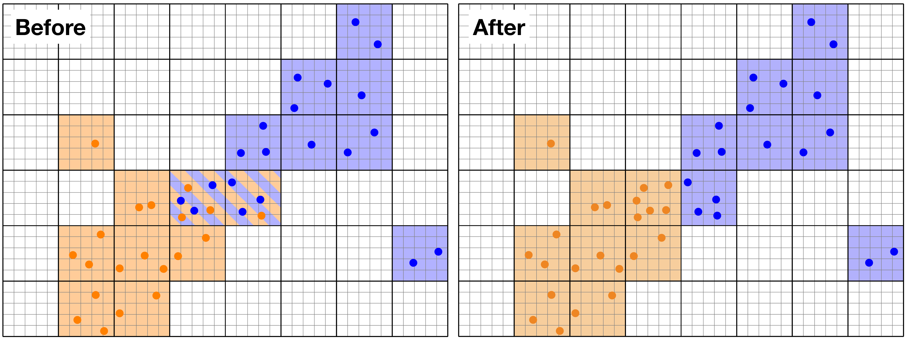Example of load-balancing for Particles. The domain is chunked along the thick lines, and the orange and blue particles are on separate MPI processors. Before load-balancing (left panel), two chuncks in the centre of the domain have both orange and blue particles. After the load-balancing (right panel), the Particles are redistributed over the processors so that the number of chunks and particles per processor is optimised.

The difficulty is that since we don’t know how the ParticleSet will disperse over time, we need to do this load-balancing ‘on the fly’. If you to contribute to the optimisation of the load-balancing, please leave a message on github!