Curvilinear grids

Parcels also supports curvilinear grids such as those used in the NEMO models.

We will be using the example data in the NemoCurvilinear_data/ directory. These fields are a purely zonal flow on an aqua-planet (so zonal-velocity is 1 m/s and meridional-velocity is 0 m/s everywhere, and no land). However, because of the curvilinear grid, the U and V fields vary north of 20N.

from datetime import timedelta as delta

import matplotlib.pyplot as plt
import numpy as np
import xarray as xr

from parcels import (
    AdvectionRK4,
    FieldSet,
    JITParticle,
    ParticleFile,
    ParticleSet,
    download_example_dataset,
)

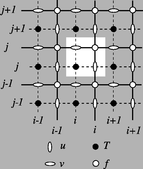
We can create a FieldSet just like we do for normal grids. Note that NEMO is discretised on a C-grid. U and V velocities are not located on the same nodes (see https://www.nemo-ocean.eu/doc/node19.html ).

 __V1__
|      |
U0     U1
|__V0__|

To interpolate U, V velocities on the C-grid, Parcels needs to read the f-nodes, which are located on the corners of the cells (for indexing details: https://www.nemo-ocean.eu/doc/img360.png ).

example_dataset_folder = download_example_dataset("NemoCurvilinear_data")
filenames = {
    "U": {
        "lon": f"{example_dataset_folder}/mesh_mask.nc4",
        "lat": f"{example_dataset_folder}/mesh_mask.nc4",
        "data": f"{example_dataset_folder}/U_purely_zonal-ORCA025_grid_U.nc4",
    },
    "V": {
        "lon": f"{example_dataset_folder}/mesh_mask.nc4",
        "lat": f"{example_dataset_folder}/mesh_mask.nc4",
        "data": f"{example_dataset_folder}/V_purely_zonal-ORCA025_grid_V.nc4",
    },
}
variables = {"U": "U", "V": "V"}

dimensions = {"lon": "glamf", "lat": "gphif", "time": "time_counter"}

fieldset = FieldSet.from_nemo(
    filenames, variables, dimensions, allow_time_extrapolation=True
)

And we can plot the U field.

plt.pcolormesh(
    fieldset.U.grid.lon,
    fieldset.U.grid.lat,
    fieldset.U.data[0, :, :],
    vmin=0,
    vmax=1,
)
plt.colorbar()
plt.show()

/var/folders/1n/500ln6w97859_nqq86vwpl000000gr/T/ipykernel_24135/4022207771.py:1: UserWarning: The input coordinates to pcolormesh are interpreted as cell centers, but are not monotonically increasing or decreasing. This may lead to incorrectly calculated cell edges, in which case, please supply explicit cell edges to pcolormesh.
  plt.pcolormesh(

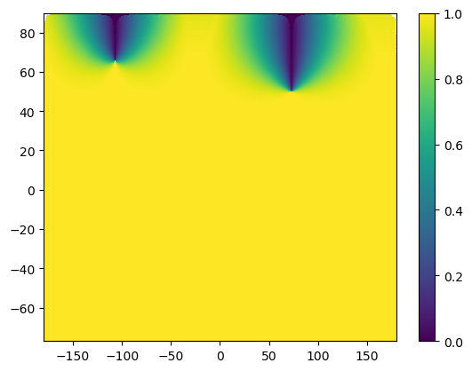
As you see above, the U field indeed is 1 m/s south of 20N, but varies with longitude and latitude north of that. We can confirm by doing a field evaluation at (60N, 50E):

u, v = fieldset.UV.eval(0, 0, 60, 50, applyConversion=False)
print(f"(u, v) = ({u:.3f}, {v:.3f})")
assert np.isclose(u, 1.0, atol=1e-3)

(u, v) = (1.000, -0.000)

Now we can run particles as normal. Parcels will take care to rotate the U and V fields.

# Start 20 particles on a meridional line at 180W
npart = 20
lonp = -180 * np.ones(npart)
latp = [i for i in np.linspace(-70, 85, npart)]

pset = ParticleSet.from_list(fieldset, JITParticle, lon=lonp, lat=latp)
pfile = ParticleFile("nemo_particles", pset, outputdt=delta(days=1))

pset.execute(AdvectionRK4, runtime=delta(days=30), dt=delta(hours=6), output_file=pfile)

INFO: Output files are stored in nemo_particles.zarr.
100%|██████████| 2592000.0/2592000.0 [00:00<00:00, 4185822.54it/s]

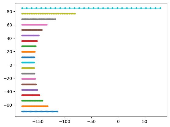
And then we can plot these trajectories. As expected, all trajectories go exactly zonal and due to the curvature of the earth, ones at higher latitude move more degrees eastward (even though the distance in km is equal for all particles).

ds = xr.open_zarr("nemo_particles.zarr")

plt.plot(ds.lon.T, ds.lat.T, ".-")
plt.show()

Speeding up ParticleSet initialisation by efficiently finding particle start-locations on the Grid

On a Curvilinear grid, determining the location of each Particle on the grid is more complicated and therefore takes longer than on a Rectilinear grid. Since Parcels version 2.2.2, a function is available on the ParticleSet class, that speeds up the look-up. After creating the ParticleSet, but before running the ParticleSet.execute(), simply call the function ParticleSet.populate_indices(). Note that this only works if you have the pykdtree package installed, which is only included in the Parcels dependencies in version >= 2.2.2

pset = ParticleSet.from_list(fieldset, JITParticle, lon=lonp, lat=latp)
pset.populate_indices()